Finite-Volume-Method on Median-Dual Meshes

The Finite Volume Method is a numerical method for the discretization of conversation laws. In this document a vertex centered FVM on median dual meshes is derived.

Problem formulation

We start with the advection equation describing the transport of some fluid, e.g. air, with density \(\rho(t, \mathbf{x}) \in \mathbb{R}\) and velocity \(\mathbf{v}(\mathbf{x}) \in \mathbb{R}^2\).

\[\begin{align*} \frac{\partial \rho}{\partial t} + \nabla \cdot (\rho v) &= 0 \text{ on } \Omega \end{align*}\]

After integrating over a yet to be specified control volume \(\mathcal{V}_i\) and application of Gauss’s divergence theorem we arrive at the following integral formulation

\[\begin{split}\begin{align} \int_{\mathcal{V}_i} \frac{\partial \rho}{\partial t} \mathrm{\,dV} + \int_{\mathcal{V}_i} \nabla \cdot (\rho \mathbf{v}) \mathrm{\,dV} &= 0 \\ \Leftrightarrow \int_{\mathcal{V}_i} \frac{\partial \rho}{\partial t} \mathrm{\,dV} + \int_{\partial {\mathcal{V}_i}} \rho \mathbf{v} \cdot \mathbf{n} \mathrm{\,dA} &= 0 \end{align}\end{split}\]

where \(n(\mathbf{x})\) is the outward surface normal. This form allows for an intuitive interpretation where the change in density inside the control volume is equal to the flux through its surface.

\[\begin{align} \int_{\mathcal{V}_i} \frac{\partial \rho}{\partial t} \mathrm{\,dV} = - \int_{\partial {\mathcal{V}_i}} \rho \mathbf{v} \cdot \mathbf{n} \mathrm{\,dA} \end{align}\]

Temporal discretization

For simplicity we consider a uniform discretization in time with time step \(\delta t\) and integrate over a single time step from time \(t^n = n \cdot \delta t\) to \(t^{n+1}\).

\[\begin{align} \int_{t^n}^{t^{n+1}} \int_{\mathcal{V}_i} \frac{\partial \rho}{\partial t} \mathrm{\,dV} \mathrm{\,dt} + \int_{t^n}^{t^{n+1}} \int_{\partial {\mathcal{V}_i}} \rho \mathbf{v} \cdot \mathbf{n} \mathrm{\,dA} \mathrm{\,dt} &= 0 \end{align}\]

After observing that the first term is nothing else but the change in density from \(t^n\) to \(t^{n+1}\) the first temporal integral collapses to a finite difference. For the surface integral term we make the first approximation by assuming the density \(\rho\) as well as the velocity at each point are approximately constant over a single time step, i.e.

\[\forall t \in [t_n, t_{n+1}] : \rho(t, \mathbf{x}) \approx \rho^n(\mathbf{x}) = \rho(t_n, \mathbf{x})\]

to obtain the following semi-discrete form

\[\begin{align} \int_{\mathcal{V}_i} (\rho^{n+1}-\rho^n) \mathrm{\,dV} + \delta t \int_{\partial {\mathcal{V}_i}} \rho^n \mathbf{v} \cdot \mathbf{n} \mathrm{\,dA} &= 0 \end{align}\]

In order the simplify notation we further introduce the average cell density \(\bar \rho_i^n\)

\[\bar \rho_i^n = \frac{1}{|\mathcal{V}_i|} \int_{\mathcal{V}_i} \rho^n \mathrm{\,dV}\]

resulting in the following time stepping scheme

\[\begin{align} \bar \rho^{n+1} = \bar \rho^{n} - \frac{\delta t}{|\mathcal{V}_i|} \int_{\partial {\mathcal{V}_i}} \rho^n \mathbf{v} \cdot \mathbf{n} \mathrm{\,dA} \end{align}\]

which again allows for an intuitive interpretation: The average density inside the control volume in the next time step is equal to average density in the last time step plus the inward-flux through the control volumes surface.

Spatial discretization

Up until now we have just considered a single control volume without actually talking about what quantities we are solving for nor the relation of the control volumes to each other. In doing so we introduce the concept of a mesh, representing a subdivision of the domain \(\Omega\) into a set of cells, either triangles or quadrilaterals.

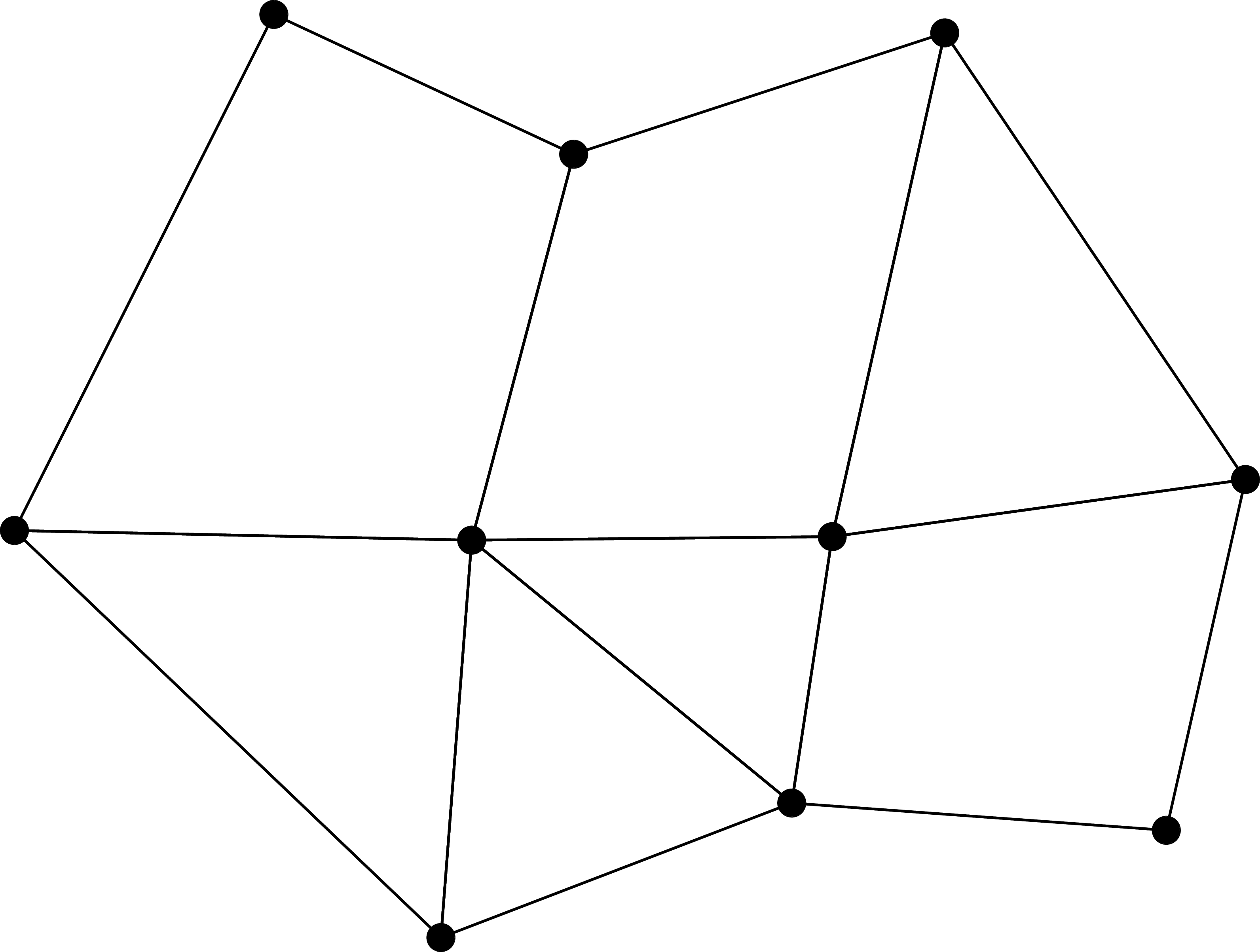
Schematic of a 2D mesh

At this point different choices for the quantities to be solved for are possible. We will here use a vertex-centered approach where the unknowns are choosen to be the densities at the vertices of the mesh \(\rho_i^n = \rho^n_i(x_i)\), which are a first order approximation of the average cell density \(\bar \rho_i^n\) appearing in the time discretized form above.

\[\begin{align} \rho_i^{n+1} &= \rho_i^{n} - \frac{\delta t}{|\mathcal{V}_i|} \int_{\partial {\mathcal{V}_i}} \rho^n \mathbf{v} \cdot \mathbf{n} \mathrm{\,dA} \end{align}\]

The control volumes \(\mathcal{V}_i\) are then constructed by joining the (bary)centers of the cells adjacent to each vertex with the midpoint of the adjacent edges. The set of control volumes form another mesh, denoted the dual mesh.

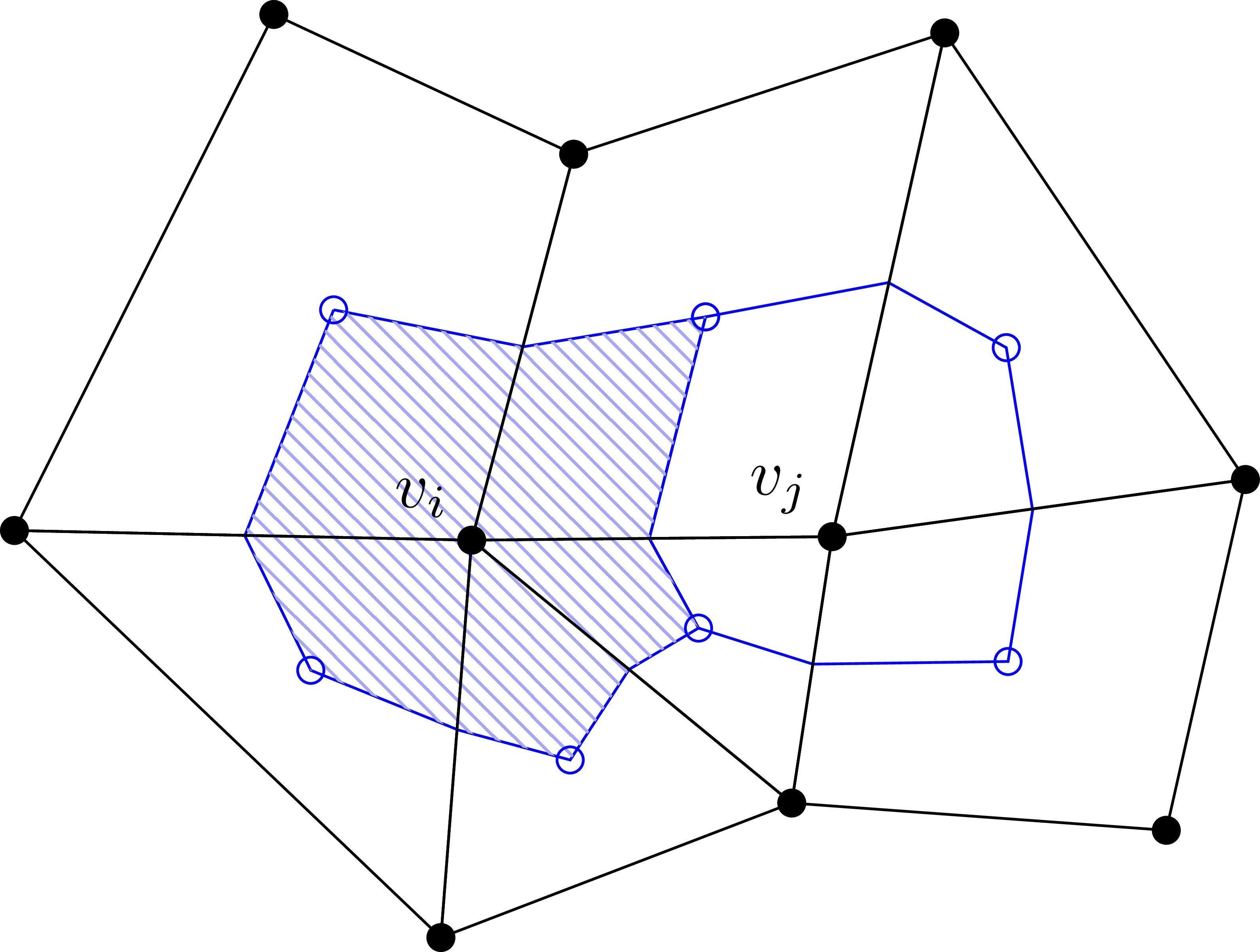
Schematic of the median-dual mesh in 2D. Primary mesh in black, dual mesh in blue. The control volume \(\mathcal{V}_i\) around the vertex \(v_i\) is constructed by joining the (bary)centers of adjacent cells with the midpoint of the outgoing edges of \(v_i\).

It remains to derive a discrete representation for the surface integral by first splitting the integral into its contributions on a set of segments \(S_j\), where each segment can be attributed to the edges adjacent to \(v_i\). Let \(|\mathcal{V}_i|\) be the area of the control volume and \(l(i)\) the number of edges adjacent to \(v_i\) then

\[\begin{align} \rho_i^{n+1} &= \rho_i^{n} - \frac{\delta t}{|\mathcal{V}_i|} \sum_{j=1}^{l(i)} \int_{S_j} \rho^n \mathbf{v} \cdot \mathbf{n} \, \mathrm{dA} \end{align}\]

The segment itself consists of the two dual edges adjacent to a primary edge from \(v_i\) to \(v_j\) and its length \(S_j\) and normal \(\mathbf{n}_j\) are approximated by

\[\begin{split}\begin{align} \mathbf{S}_j &= (\mathbf{c}_{1}-\mathbf{c}_{2}) \cdot (\begin{bmatrix} 0 & 1 \\ -1 & 0 \\ \end{bmatrix}) \\ S_j &= ||\mathbf{S}_j||_2 \\ \mathbf{n}_j &= \frac{\mathbf{S}_j}{S_j} \end{align}\end{split}\]

with \(\mathbf{c}_{1}\) and \(\mathbf{c}_{2}\) the coordinates of the two bary(centers).

Lastly to ensure stability of the method the flux density perpendicular to the surface \(F_i^\perp = \rho^n \mathbf{v} \cdot \mathbf{n}\) is approximated by a simple upwind flux

\[F_i^\perp(\rho_i, \rho_j, v) \approx [v_j^\perp]^+ \rho_i + [v_j^\perp]^- \rho_j\]

where \(v_j^\perp = \mathbf{v} \cdot n_j\) is the normal velocity evaluated at the surface \(S_j\) and its positive and negative parts are defined as

\[\begin{split}[V^\perp]^+ = \mathrm{max}(0, V^\perp) \\ [V^\perp]^- = \mathrm{min}(0, V^\perp)\end{split}\]

The resulting fully discrete time stepping scheme then reads

\[\begin{align} \rho_i^{n+1} &= \rho_i^{n} - \frac{\delta t}{|\mathcal{V}_i|} \sum_{j=1}^{l(i)} F_j^\perp S_j \end{align}\]

Implementation in GT4Py

To be written.

TODO

Frame extension to IFS-FVM

• curvilinear coordinates

• pseudo velocity (higher order spatial discretization)

• additional differential operators (higher order temporal)

• adaptive time stepping

• CFL

Notes

Code for the construction of the dual mesh in Atlas: src/atlas/mesh/actions/BuildDualMesh.cc