Getting Started
This chapter describes how to use GridTools to solve a (simple) PDE. We will use a fourth-order horizontal smoothing filter to explain the necessary steps to assemble a stencil from scratch. We will not go into details in this chapter but refer to later chapters for more details.
Our example PDE is given by
where \(\nabla^4\) is the squared two dimensional horizontal Laplacian and we apply the filter only up to some maximal \(z_0\) (to make the example more interesting). The filter is calculated in two steps: first we calculate the Laplacian of \(\phi\)
then we calculate the Laplacian of \(L\) as \(-\alpha \nabla^4 \phi = -\alpha \Delta L\).
In the following we will walk through the following steps:
The GridTools coordinate system and its notation.
Storages: how does GridTools manage the input and output fields.
The first stencil: calculating \(L\), the second order Laplacian of \(\phi\).
The final stencil: function calls, apply-method overloads and temporaries
Coordinate System
For a finite difference discretization we restrict the field \(\phi \in \mathbb{R}^3\) to a discrete grid. We use the notation \(i = x_i\) and \(j = y_j\) for the horizontal dimension and \(k = z_k\) for the vertical dimension, where \(x_i, y_j, z_k\) are the \(x,y,z\) coordinates restricted on the grid. The computation domain is defined by all grid points in our domain of interest
GridTools supports any number of dimension, however the iteration is always restricted to three dimensions, and GridTools will treat one dimension, here the \(k\) dimension, differently: the \(ij\)-plane is executed in parallel while the computation in \(k\) can be sequential. The consequence is that there must not be a dependency in \(ij\) within a stencil while there can be a dependency in \(k\). For now (this chapter) it is sufficient to just remember that the \(ij\)-plane and the \(k\) dimension are treated differently by GridTools.
The calculation domain is surrounded by a boundary region as depicted in Fig. 1. Computation happens only within the calculation domain but values may be read from grid points in the boundary region.
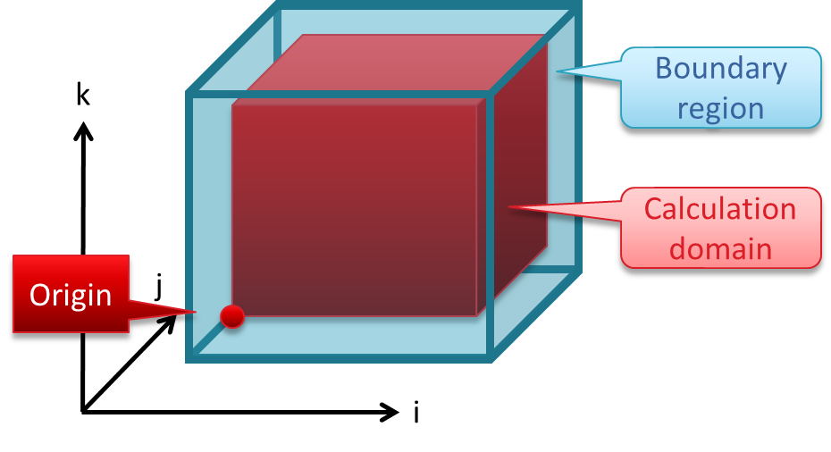
Fig. 1 Coordinate system
Storages
In this section we will set up the fields for our example: we need a
storage for the \(\phi\)-field (phi_in) and a storage for the output
(phi_out).
Storages in GridTools are n-dimensional array-like objects with the following capabilities:
access an element with \((i,j,k)\) syntax
synchronization between CPU memory and a device (e.g. a CUDA capable GPU)
Storage Traits
Since the storages depend on the architecture (e.g. CPU or GPU) our first step is to define the storage traits type which typically looks like
#include <gridtools/storage/gpu.hpp>
using traits_t = storage::gpu;
for the CUDA Storage Traits or
#include <gridtools/storage/cpu_ifirst.hpp>
using traits_t = storage::cpu_ifirst;
for the CPU Storage Traits.
Building Storages
For efficient memory accesses the index ordering might depend on the target architecture, therefore the memory layout will be implicitly decided by storage traits.
GridTools storage classes don’t have user facing constructors. The builder design pattern is used instead.
The library provides the storage::builder object template that is instantiated by storage traits.
To create a storage we need to supply the builder with the desired storage properties by chaining
the setter methods and finally call the build() method which returns a std::shared_ptr
of a newly created storage. The builder also provides overloaded call operator which is a synonym of build().
There are two required properties that need to be set:
the type of element, eg .type<double>(), and the sizes for each dimension, eg .dimensions(10, 12, 20).
Other properties are optional.
If we need several storages that share some properties, we can construct a partially specified builder by setting the shared properties and reuse it while building concrete storages.
uint_t Ni = 10;
uint_t Nj = 12;
uint_t Nk = 20;

auto const builder = storage::builder<traits_t>.dimensions(Ni, Nj, Nk).id<0>();
auto phi = builder
               .name("phi")                                                //
               .type<float>()                                              //
               .initializer([](int i, int j, int k) { return i + j + k; }) //
               .build();
auto lap = builder.name("lap").type<double>().value(-1).build();
Note
It is recommended to use the id property each time the dimensions property is set.
id should identify the unique set of dimension sizes.
This is because the stencil computation engine assumes that the storages that have the same id have the same
sizes. However, if only one set of dimensions is used, the id property can be skipped.
We can now
retrieve the name of the field,
create a view and read and write values in the field using the parenthesis syntax,
query the lengths of each dimension.
std::cout << phi->name() << "\n";

auto phi_view = phi->host_view();
phi_view(1, 2, 3) = 3.1415;
std::cout << "phi_view(1, 2, 3) = " << phi_view(1, 2, 3) << std::endl;
std::cout << "j length = " << phi->lengths()[1] << std::endl;
Stencils
A stencil is a kernel that updates array elements according to a fixed access pattern.
Example: Naive 2D Laplacian
The simplest discretization of the 2D Laplacian is the finite difference five-point stencil as depicted in Fig. 2.
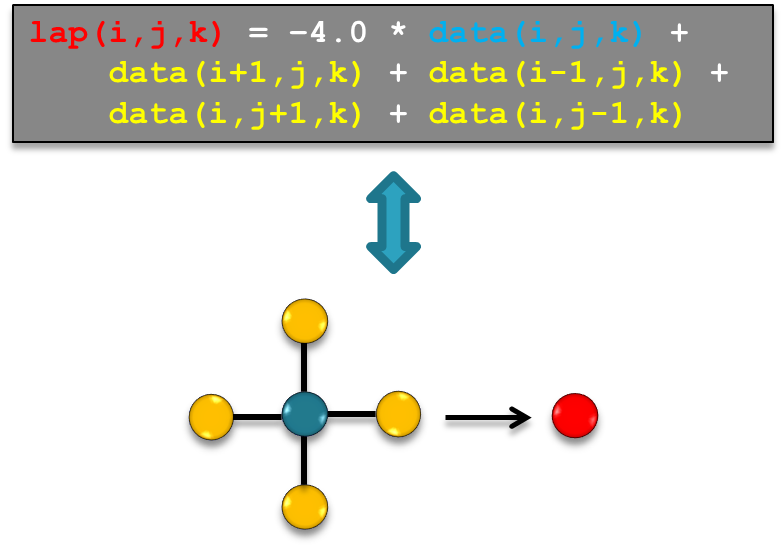
Fig. 2 Access pattern of a 2D Laplacian
For the calculation of the Laplacian at a given grid point we need the value at the grid point itself and its four direct neighbors along the Cartesian axis.
A naive C++ implementation of the 2D Laplacian stencil looks as follows:
auto laplacian = [](auto &lap, auto &in, int boundary_size) {
    auto lengths = in.lengths();
    int Ni = lengths[0];
    int Nj = lengths[1];
    int Nk = lengths[2];
    for (int i = boundary_size; i < Ni - boundary_size; ++i) {
        for (int j = boundary_size; j < Nj - boundary_size; ++j) {
            for (int k = boundary_size; k < Nk - boundary_size; ++k) {
                lap(i, j, k) = -4.0 * in(i, j, k)                  //
                               + in(i + 1, j, k) + in(i - 1, j, k) //
                               + in(i, j + 1, k) + in(i, j - 1, k);
            }
        }
    }
};
Apart from the initialization the stencil implementation consists of 2 main components:
Loop-logic: defines the stencil application domain and loop order
Update-logic: defines the update formula (here: the 2D Laplacian)
Special care has to be taken at the boundary of the domain. Since the Laplacian needs the neighboring points, we cannot calculate the Laplacian on the boundary layer and have to exclude it from the loop.
First GridTools Stencil
In GridTools the loop logic and the storage order are implemented (and optimized) by the library while the update function, to be applied to each gridpoint, is implemented by the user. The loop logic (for a given architecture) is combined with the user-defined update function at compile-time by template meta-programming.
Update-logic: GridTools 2D Laplacian
The update-logic is implemented with state-less functors. A
GridTools functor is a struct or class providing a static method
called apply. The update-logic is implemented in these Apply-Methods.
As the functors are state-less (no member variables, static methods
only) they can be passed by type, i.e. at compile-time, and therefore
allow for compile-time optimizations.
struct lap_function {
    using in = in_accessor<0, extent<-1, 1, -1, 1>>;
    using lap = inout_accessor<1>;

    using param_list = make_param_list<in, lap>;

    template <typename Evaluation>
    GT_FUNCTION static void apply(Evaluation &&eval) {
        eval(lap()) = eval(-4. * in() + in(1, 0) + in(0, 1) + in(-1, 0) + in(0, -1));
    }
};
In addition to the apply-method, the functor contains accessor s. These
two accessor s are parameters of the functor, i.e. they are mapped to
fields passed to the functor. They contain compile-time information if
they are only used as input parameters, e.g. the in accessor in the
example, or if we want to write into the associated field (inout). Additionally,
the extent defines which grid points are needed by the stencil relative
to the current point. The format for the extent is
extent<i_minus, i_plus, j_minus, j_plus, k_minus, k_plus>
where i_minus and i_plus define an interval on the \(i\)-axis relative to
the current position; i_minus is the negative offset, i.e. zero or a
negative number, while i_plus is the positive offset. Analogously for
\(j\) and \(k\). In the Laplacian example, the first two numbers
in the extent of the in accessor define that we want to access the
field at \(i-1\), \(i\) and \(i+1\). The accessor type and the extent is needed for a
dependency analysis in the compile-time optimizations for more complex
stencils. (For example, the computation
domain needs to be extended when we calculate the Laplacian of the Laplacian later. This is done automatically by the
library.)
The first template argument is an index defining the order of the
parameters, i.e. the order in which the fields are passed to the
functor. The param_list is a GridTools keyword which has to be defined for each stencil,
and should contain the list of accessors.
A apply-method needs as first parameter a context
object, usually called eval, which is created and passed to the method by the library on
invocation. This object contains, among other things, the index of the
active grid point (Iteration Point) and the mapping of data-pointers to the accessor s. The
second argument is optional and specifies the interval on the \(k\)-axis where this implementation
of the Apply-Method should be executed. This allows to apply a different update-logic on
Vertical Intervals by overloading the Apply-Method. We will define Vertical Intervals
later. If the second parameter is not specified, a default interval is assumed.
The body of the apply-method looks quite similar to the one in the
naive implementation, except that each
field access has to be wrapped by a call to the context object eval.
This is necessary to map the compile-time parameter, the accessor, to
the run-time data in the data_store.
Calling the Stencil
In the naive implementation, the call to the laplacian is as simple as
int boundary_size = 1;
laplacian( lap, phi, boundary_size );
since it contains already all the information: the update-logic and the loop-logic.
The GridTools stencil, does not contain any information about the loop-logic, i.e. about the domain where we want to apply the stencil operation, since we need to specify it in a platform-independent syntax, a domain specific embedded language (DSEL), such that the Backend can decide on the specific implementation.
For our example this looks as follows
 1uint_t Ni = 10;
 2uint_t Nj = 12;
 3uint_t Nk = 20;
 4int halo = 1;
 5
 6auto builder = storage::builder<storage_traits_t> //
 7                   .type<double>()                //
 8                   .dimensions(Ni, Nj, Nk)        //
 9                   .halos(halo, halo, 0);         //
10
11auto phi = builder();
12auto lap = builder();
13
14halo_descriptor boundary_i(halo, halo, halo, Ni - halo - 1, Ni);
15halo_descriptor boundary_j(halo, halo, halo, Nj - halo - 1, Nj);
16auto grid = make_grid(boundary_i, boundary_j, Nk);
17
18run_single_stage(lap_function(), stencil_backend_t(), grid, phi, lap);
In lines 14-16 we setup the physical dimension of the problem. First we define which points on the \(i\) and the \(j\)-axis belong to the computational domain and which points belong to the boundary (or a padding region). For now it is enough to know that these lines define a region with a boundary of size 1 surrounding the \(ij\)-plane. In the next lines the layers in \(k\) are defined. In this case we have only one interval. We will discuss the details later.
In line 18 we execute the stencil computation. In our example only one stencil participates.
Hence, we can use the simple run_single_stage API. We pass the stencil the backend object, the grid
(the information about the loop bounds) and the storages on which the computation needs to be executed.
The number and the order of storage arguments should match the number of stencil accessors.
Full GridTools Laplacian
The full working example looks as follows:
 1/*
 2 * GridTools
 3 *
 4 * Copyright (c) 2014-2021, ETH Zurich
 5 * All rights reserved.
 6 *
 7 * Please, refer to the LICENSE file in the root directory.
 8 * SPDX-License-Identifier: BSD-3-Clause
 9 */
10#include <gridtools/common/defs.hpp>
11#include <gridtools/stencil/cartesian.hpp>
12#include <gridtools/storage/builder.hpp>
13#include <gridtools/storage/sid.hpp>
14
15using namespace gridtools;
16using namespace stencil;
17using namespace cartesian;
18using namespace expressions;
19
20#ifdef GT_CUDACC
21#include <gridtools/stencil/gpu.hpp>
22#include <gridtools/storage/gpu.hpp>
23using stencil_backend_t = stencil::gpu<>;
24using storage_traits_t = storage::gpu;
25#else
26#include <gridtools/stencil/cpu_ifirst.hpp>
27#include <gridtools/storage/cpu_ifirst.hpp>
28using stencil_backend_t = stencil::cpu_ifirst<>;
29using storage_traits_t = storage::cpu_ifirst;
30#endif
31
32struct lap_function {
33    using in = in_accessor<0, extent<-1, 1, -1, 1>>;
34    using lap = inout_accessor<1>;
35
36    using param_list = make_param_list<in, lap>;
37
38    template <typename Evaluation>
39    GT_FUNCTION static void apply(Evaluation &&eval) {
40        eval(lap()) = eval(-4. * in() + in(1, 0) + in(0, 1) + in(-1, 0) + in(0, -1));
41    }
42};
43
44int main() {
45    uint_t Ni = 10;
46    uint_t Nj = 12;
47    uint_t Nk = 20;
48    int halo = 1;
49
50    auto builder = storage::builder<storage_traits_t> //
51                       .type<double>()                //
52                       .dimensions(Ni, Nj, Nk)        //
53                       .halos(halo, halo, 0);         //
54
55    auto phi = builder();
56    auto lap = builder();
57
58    halo_descriptor boundary_i(halo, halo, halo, Ni - halo - 1, Ni);
59    halo_descriptor boundary_j(halo, halo, halo, Nj - halo - 1, Nj);
60    auto grid = make_grid(boundary_i, boundary_j, Nk);
61
62    run_single_stage(lap_function(), stencil_backend_t(), grid, phi, lap);
63}
There are some points which we did not discuss so far. For a first look at GridTools these can be considered fixed patterns and we won’t discuss them now in detail.
A common pattern is to use the preprocessor flag __CUDACC__ to distinguish between CPU and GPU code.
Here we use the GridTools internal GT_CUDA macro to do this. The macro is used to set the correct Backend
and Storage Traits for the CUDA or CPU architecture, respectively.
The code example can be compiled using the following simple CMake script (requires an installation of GridTools, see Installing and Validating GridTools).
cmake_minimum_required(VERSION 3.14.5)

project(GridTools-laplacian LANGUAGES CXX)

set(CMAKE_CXX_EXTENSIONS OFF) # Currently required for HIP

find_package(GridTools 2.2.0 REQUIRED QUIET)

if(TARGET GridTools::stencil_cpu_ifirst)
    add_executable(gt_laplacian test_gt_laplacian.cpp)
    target_link_libraries(gt_laplacian GridTools::gridtools GridTools::stencil_cpu_ifirst)
endif()
Assembling Stencils: Smoothing Filter
In the preceding section we saw how a first simple GridTools stencil is defined and executed. In this section we will use this stencil to compute our example PDE. A naive implementation could look as in
auto naive_smoothing = [](auto &out, auto &in, double alpha, int kmax) {
    int lap_boundary = 1;
    int full_boundary = 2;

    int Ni = in.lengths()[0];
    int Nj = in.lengths()[1];
    int Nk = in.lengths()[2];

    // Instantiate temporary fields
    auto make_storage = storage_builder.dimensions(Ni, Nj, Nk);
    auto lap_storage = make_storage();
    auto lap = lap_storage->target_view();
    auto laplap_storage = make_storage();
    auto laplap = laplap_storage->target_view();

    // laplacian of phi
    laplacian(lap, in, lap_boundary);
    // laplacian of lap
    laplacian(laplap, lap, full_boundary);

    for (int i = full_boundary; i < Ni - full_boundary; ++i) {
        for (int j = full_boundary; j < Nj - full_boundary; ++j) {
            for (int k = full_boundary; k < Nk - full_boundary; ++k) {
                if (k < kmax)
                    out(i, j, k) = in(i, j, k) - alpha * laplap(i, j, k);
                else
                    out(i, j, k) = in(i, j, k);
            }
        }
    }
};
For the GridTools implementation we will learn three things in this section: how to define special regions in the \(k\)-direction; how to use GridTools temporaries and how to call functors from functors.
apply-method overload
Our first GridTools implementation will be very close to the naive implementation: we will call two times the Laplacian functor from the previous section and store the result in two extra fields. Then we will call a third functor to compute the final result. This functor shows how we can specialize the computation in the \(k\)-direction:
struct smoothing_function_1 {
    using phi = in_accessor<0>;
    using laplap = in_accessor<1>;
    using out = inout_accessor<2>;

    using param_list = make_param_list<phi, laplap, out>;

    constexpr static double alpha = 0.5;

    template <typename Evaluation>
    GT_FUNCTION static void apply(Evaluation &eval, lower_domain) {
        eval(out()) = eval(phi() - alpha * laplap());
    }

    template <typename Evaluation>
    GT_FUNCTION static void apply(Evaluation &eval, upper_domain) {
        eval(out()) = eval(phi());
    }
};
We use two different
Vertical Intervals, the lower_domain and the upper_domain, and provide an overload of the
Apply-Method for each interval.
The Vertical Intervals are defined as
using axis_t = axis<2>;
using lower_domain = axis_t::get_interval<0>;
using upper_domain = axis_t::get_interval<1>;
The first line defines an axis with 2 Vertical Intervals. From this axis retrieve the Vertical Intervals and give them a name.
Then we can assemble the computation
auto phi = make_storage();
auto phi_new = make_storage();
auto lap = make_storage();
auto laplap = make_storage();

halo_descriptor boundary_i(halo, halo, halo, Ni - halo - 1, Ni);
halo_descriptor boundary_j(halo, halo, halo, Nj - halo - 1, Nj);
auto grid = make_grid(boundary_i, boundary_j, axis_t(kmax, Nk - kmax));

auto const spec = [](auto phi, auto phi_new, auto lap, auto laplap) {
    return execute_parallel()
        .stage(lap_function(), phi, lap)
        .stage(lap_function(), lap, laplap)
        .stage(smoothing_function_1(), phi, laplap, phi_new);
};

run(spec, stencil_backend_t(), grid, phi, phi_new, lap, laplap);
We cannot use the run_single_stage API because now we need to compose a Computation from three stencil calls. To achieve that
we use the full featured run API. It requires a stencil composition specification as a first parameter. That specification
is provided in form of a generic lambda. Its arguments represent the storages that are used in the computation.
The expression that is returned describes how the stencils should be composed. It is where the GridTools DSL is used.
execute_parallel() means that each \(k\)-level can be executed in parallel. The stage clause represents
a call to the stencil with the given arguments.
In this version we needed to explicitly allocate the temporary fields
lap and laplap. In the next section we will learn about
GridTools temporaries.
GridTools Temporaries
GridTools temporary storages are storages with the lifetime of the
computation. This is exactly what we need for the lap and laplap
fields.
Note
Note that temporaries are not allocated explicitly and we cannot access them from outside of the computation. Therefore, sometimes it might be necessary to replace a temporary by a normal storage for debugging.
To use temporary storages we exclude the correspondent fields from the arguments of our spec and declare them as
temporaries, within the spec lambda, using the GT_DECLARE_TMP macro. We don’t need the explicit
instantiations any more and don’t have to pass them to the run. The new code looks as follows
auto phi = make_storage();
auto phi_new = make_storage();

halo_descriptor boundary_i(halo, halo, halo, Ni - halo - 1, Ni);
halo_descriptor boundary_j(halo, halo, halo, Nj - halo - 1, Nj);
auto grid = make_grid(boundary_i, boundary_j, axis_t{kmax, Nk - kmax});

auto const spec = [](auto phi, auto phi_new) {
    GT_DECLARE_TMP(double, lap, laplap);
    return execute_parallel()
        .stage(lap_function(), phi, lap)
        .stage(lap_function(), lap, laplap)
        .stage(smoothing_function_1(), phi, laplap, phi_new);
};

run(spec, stencil_backend_t(), grid, phi, phi_new);
Besides the simplifications in the code (no explicit storage needed), the concept of temporaries allows GridTools to apply optimization. While normal storages have a fixed size, temporaries can have block-private Halos which are used for redundant computation.
Note
It might be semantically incorrect to replace a temporary with a normal storage, as normal storages don’t have the Halo region for redundant computation. In such case several threads (OpenMP or CUDA) will write the same location multiple times. As long as all threads write the same data (which is a requirement for correctness of GridTools), this should be no problem for correctness on current hardware (might change in the future) but might have side-effects on performance.
Note
This change from normal storages to temporaries did not require any code changes to the functor.
Functor Calls
The next feature we want to use is the stencil function call. In the first example we computed the Laplacian and the Laplacian of the Laplacian explicitly and stored the intermediate values in the temporaries. Stencil function calls will allow us do the computation on the fly and will allow us to get rid of the temporaries.
Note
Note that this is not necessarily a performance optimization. It might well be that the version with temporaries is actually the faster one.
In the following we will remove only one of the temporaries. Instead of calling the Laplacian twice from the
spec, we will move one of the calls into the smoothing functor. The new smoothing functor looks as follows
struct smoothing_function_3 {
    using phi = in_accessor<0>;
    using lap = in_accessor<1, extent<-1, 1, -1, 1>>;
    using out = inout_accessor<2>;

    using param_list = make_param_list<phi, lap, out>;

    constexpr static double alpha = 0.5;

    template <typename Evaluation>
    GT_FUNCTION static void apply(Evaluation &eval, lower_domain) {
        eval(out()) = eval(phi() - alpha * call<lap_function>::with(eval, lap()));
    }

    template <typename Evaluation>
    GT_FUNCTION static void apply(Evaluation &eval, upper_domain) {
        eval(out()) = eval(phi());
    }
};
In call we specify the functor which we want to apply. In with the eval is forwarded, followed by all the
input arguments for the functor. The functor in the call is required to have exactly one inout_accessor which will
be the return value of the call. Note that smoothing_function_3 still needs to specify the extents explicitly;
for functor calls they cannot be inferred automatically.
One of the stage(lap_function(), ...) was now moved inside of the functor, therefore the new spec is just:
auto phi = make_storage();
auto phi_new = make_storage();

halo_descriptor boundary_i(halo, halo, halo, Ni - halo - 1, Ni);
halo_descriptor boundary_j(halo, halo, halo, Nj - halo - 1, Nj);
auto grid = make_grid(boundary_i, boundary_j, axis_t{kmax, Nk - kmax});

auto const spec = [](auto phi, auto phi_new) {
    GT_DECLARE_TMP(double, lap);
    return execute_parallel()                              //
        .stage(lap_function(), phi, lap)                   //
        .stage(smoothing_function_3(), phi, lap, phi_new); //
};

run(spec, stencil_backend_t(), grid, phi, phi_new);
The attentive reader may have noticed that our first versions did more work than needed: we calculated the Laplacian of the Laplacian of phi (\(\Delta \Delta \phi\)) for all \(k\)-levels, however we used it only for \(k<k_\text{max}\). In this version we do a bit better: we still calculate the Laplacian (\(L = \Delta \phi\)) for all levels but we only calculate \(\Delta L\) for the levels where we need it.