User Manual

Storage Library

The Storage Library provides the way to represent multidimensional typed contiguous memory allocations with arbitrary layout and alignment. All entities are defined in the gridtools::storage namespace.

Data Store

The key entity of the library, representing a multidimensional array.

• Data store has no user facing constructors. To create it one should use the Builder API.

• The access to the actual data is indirect. Data store has methods to request a view. The view provides data access via overloaded call operator.

• Data store is aware of memory spaces. It distinguish between target and host data access. Views are requested with target_view()/target_const_view()/host_view()/host_const_view() methods. If target and host spaces are different and the data store holds non constant data, data store performs automatic memory synchronization if needed. It is assumed that the target memory space access is used for doing computations and host access is used for filling, dumping and verifying the data.

Data Store Synopsis

template</* Implementation defined parameters */>
class data_store {
  public:
    static constexpr size_t ndims; /* Dimensionality */
    using layout_t = /* Instantiation of gridtools::layout_map. */;
    using data_t = /* Type of the element. */;
    // The following invariant is held: for any data_store instancies that have
    // the same kind_t the strides are also the same.
    using kind_t = /* A type that identifies the strides set. */;

    // Data store arbitrary label. Mainly for debugging.
    std::string const &name() const;
    // The sizes of the data store in each dimension.
    array<unsigned, ndims> lengths() const;
    // The strides of the data store in each dimension.
    array<unsigned, ndims> strides() const;

    // lengths and strides in the form of tuples.
    // If the length along some dimension is known in compile time (N),
    // it is represented as an intergral_constant<int, N>,
    // otherwise as int.
    auto const& native_lengths() const;
    auto const& native_strides() const;

    // 1D length of the data store expressed in number of elements.
    // Namely it is a pointer difference between the last and the first element minus one.
    unsigned length() const;

    // Supplementary object that holds lengths and strides.
    auto const &info() const;

    // Request the target view.
    // If the target and host spaces are different necessary synchronization is performed
    // and the host counterpart is marked as dirty.
    auto target_view();
    // Const version doesn't mark host counterpart as dirty. Synchronization takes place.
    auto const_target_view();

    // Raw ptr alternatives for target_view/const_target_view.
    // Synchronization behaviour is the same.
    data_t *get_target_ptr();
    data_t const *get_const_target_ptr();

    // Host access methods variations. They only exist if !std::is_const<data_t>::value.
    auto host_view();
    auto host_const_view();
    data_t *get_host_ptr();
    data_t const *get_const_host_ptr();
};

Data View Synopsis

Data view is a supplemental struct that is returned form data store access methods. The distinctive property: data view is a POD. Hence it can be passed to the target device by copying the memory. For the gpu data stores all data view methods are declared as device only.

template <class T, size_t N>
struct some_view {
    // POD members here

    // The meta info methods are the same as for data_store.
    array<unsigned, N> lengths() const;
    array<unsigned, N> strides() const;
    auto const& native_lengths() const;
    auto const& native_strides() const&
    unsigned length() const;
    auto const &info() const;

    // raw access
    T *data() const;
    // multi dimensional indexed access
    T &operator()(int... /*number of arguments equals to N*/ ) const;
    // variation with array as an argument
    T &operator()(array<int, N> const &) const;
};

Note

On data store synchronization behaviour

If target and host spaces are different and the data is mutable, data store manages both target and host allocations. Internally it keeps a flag that can be either clean, dirty target or dirty host. When a view is requested and the correspondent allocation is marked as dirty, the data store performs a memory transfer and the allocation is marked as clean. The counterpart allocation is marked as dirty if a non-constant view is requested. Each new view request potentially invalidates the previously created views. Therefore, is is best practice to limit the scope of view objects as much as possible to avoid stale data views. Here are some illustrations:

template <class View>
__global__ void kernel(View view) { view(0) = view(1) = OxDEADBEEF; }

...

// host and target allocations are made here. The state is set to clean
auto ds = builder<gpu>.type<int>().dimensions(2)();

// no memory transfer because of the clean state
// the state becomes dirty_target
auto host_view = ds->host_view();
// the use of the host view
host_view(0) = host_view(1) = 42;

// memory transfer to the target space because the state is dirty_target
// the state becomes dirty_host
// host_view becomes stale at this point
auto target_view = ds->target_view();

// the use of the target view
kernel<<<1,1>>>(target_view);

// memory transfer to the host space because the state is dirty_host
// the state becomes clean
// both host_view and target_view are stale at this point
auto host_view_2 = ds->const_host_view();
// the use of the second host view
assert(host_view_2(0) == OxDEADBEEF);
assert(host_view_2(1) == OxDEADBEEF);

We can refactor this to exclude the possibility of using state data:

{
    auto v = ds->host_view();
    v(0) = v(1) = 42;
}

kernel<<<1,1>>>(ds->target_view());

{
    auto v = ds->const_host_view();
    assert(v(0) == OxDEADBEEF);
    assert(v(1) == OxDEADBEEF);
}

Builder API

The builder design pattern is used for data store construction. The API is defined in gridtools/storage/builder.hpp. Here a single user facing symbol is defined – storage::builder. It is a value template parametrized by Traits (see below). The idea is that the user takes a builder with the desired traits, customize it with requested properties and finally calls the build() method (or alternatively the overloaded call operator) to produce a std::shared_ptr to a data store. For example:

auto ds = storage::builder<storage::gpu>
        .type<double>()
        .name("my special data")
        .dimensions(132, 132, 80)
        .halos(2, 2, 0)
        .selector<1, 1, 0>()
        .value(42)
        .build();

assert(ds->const_host_view()(1, 2, 3) == 42);

One can also use partially specified builder to produce several data stores:

auto const my_builder = storage::builder<storage::gpu>.dimensions(10, 10, 10);
auto foo = my_builder.type<int>().name("foo")();
auto bar = my_builder.type<tuple<int, double>>()();
auto baz = my_builder
         .type<double const>
         .initialize([](int i, int j, int k){ return i + j + k; })
         .build();

This API implements an advanced variation of the builder design pattern. Unlike classic builder, the setters don’t return a reference *this, but a new instance of a potentially different class. Because of that an improper usage of builder is caught at compile time:

// compilation failure: dimensions should be set
auto bad0 = builder<cpu_ifirst>.type<double>().build();

// compilation failure: value and initialize setters are mutually exclusive
auto bad1 = builder<cpu_ifirst>
          .type<int>()
          .dimensions(10)
          .value(42)
          .initialize([](int i) { return i;})
          .build();

Builder Synopsis

template </* Implementation defined parameters. */>
class buider_type {
  public:
    template <class>
    auto type() const;
    template <int>
    auto id() const;
    auto unknown_id() const;
    template <int...>
    auto layout() const;
    template <bool...>
    auto selector() const;
    auto name(std::string) const;
    auto dimensions(...) const;
    auto halos(unsigned...) const;
    template <class Fun>
    auto initializer(Fun) const;
    template <class T>
    auto value(T) const;
    auto build() const;
    auto operator()() const { return build(); }
};
template <class Traits>
constexpr builder_type</* Implementation defined parameters. */> builder = {};

Constrains on Builder Setters

• type and dimensions should be set before calling build

• any property can be set at most once

• layout and selector properties are mutually exclusive

• value and initializer properties are mutually exclusive

• the template arity of layout/selector equals dimension arity

• halos arity equals dimension arity

• initializer argument is callable with int ‘s, has dimension arity and its return type is convertible to type argument

• value argument type is convertible to type argument.

• if type argument is const, value or initializer should be set

Notes on Builder Setters Semantics

• id: The use case of setting id is to ensure the invariant for data_store::kind_t. It should identify the unique set of dimension sizes. Note the difference: data_store::kind_t represents the set of unique strides, but id represents the set of unique sizes. Example:

  // We have two different sizes that we use in our computation.
  // Hence we prepare two partially specified builders.
  auto const builder_a = builder<gpu>.id<0>.dimensions(3, 4, 5);
  auto const builder_b = builder<gpu>.id<1>.dimensions(5, 6, 7);
  
  // We use our builders to make some data_stores.
  auto a_0 = builder_a.type<double>().build();
  auto a_1 = builder_a.type<double>().build();
  auto a_2 = builder_a.type<float>().halos(1, 1, 0).build();
  auto b_0 = builder_a.type<double>().build();
  
  // kind_t aliases of a_0 and a_1 are the same.
  // kind_t aliases of a_0 and b_0 are different,
  //   because the id property is different.
  // kind_t aliases of a_0 and a_2 are different,
  //   even though id property is the same,
  //   because types are different.
  

  At the moment id/kind_t matters if data stores are used in the context of GridTools stencil computation. Otherwise there is no need to set id. Note also that setting id can be skipped if only one set of dimension sizes is used even in GridTools stencil computation context.

• unknown_id: If unknown_id is set for the builder, the resulting data_store::kind_t will be equal to sid::unknown_kind. This will opt out this data store from the optimizations that are used in the gridtools stencil computation. it makes sense to set unknown_id if the same builder is used to create the data stores with different dimension set and those fields are participating in the same stencil computation.

• dimensions: Allows to specify the dimensions of the array. Arguments are either of integral type or derived from the std::integral_constant instantiation. Examples:

  using gridtools::literals;
  auto const my_builder = builder<cpu_ifirst>.type<int>();
  auto dynamic_ds = my_builder.dimensions(2, 3)();
  auto static_ds = my_builder.dimensions(2_c, 3_c)();
  auto mixed_ds = my_builder.dimensions(2, 3_c)();
  

  In this example all data stores act almost the same way. But static_ds (unlike dynamic_ds) does not hold its dimensions in runtime, it is encoded in the type instead. I.e. meta information (lengths/strides) takes less space and also indexing/iterating code can be more aggressively optimized by compiler.

• halos: The memory alignment is controlled by specifying Traits (the template parameter of the builder). By default each first element of the innermost dimension is aligned. halos allows to explicitly specify the index of element that should be aligned. Together with chosen element, all elements that share its innermost index will be aligned as well.

• selector: allows to mask out any dimension or several. Example:

  auto ds = builder<cpu_ifirst>.type<int>().selector<1,0>().dimensions(10, 10).value(-1)();
  auto view = ds->host_view();
  // even though the second dimension is masked out
  // we can used indices in the defined range
  assert(ds->lengths()[1], 10);
  assert(view(0, 0) == -1);
  assert(view(0, 9) == -1);
  // but elements that differs only by the masked out index refer to the same data
  assert(&view(0, 1) == &view(0, 9));
  

• layout: By default the data layout is controlled by Traits. However it is overridable with the layout setter. Example:

  auto ds0 = builder<gpu>
      .type<int>()
      .layout<0, 2, 4, 1, 3>()
      .dimensions(10, 10, 10, 10, 10)
      .name("my tuned storage for the specific use case")
      .build();
  

  The template parameters of layout are a permutation of the value from 0 to N - 1, where N is the number of dimensions of the storage. The values indicate the order of the dimensions by decreasing strides. For instance a C array X[i][j][k] layout would be equivalent to .layout<0,1,2>(). The dimension with stride 1 has the highest index, so in this case, the k-stride is a unit stride. A Fortran style array X[i][j][k] layout would be equivalent to .layout<2,1,0>(), meaning that the i-stride is a unit-stride (thus, the first index of the layout is 2).

  There is also the possibility to mask dimensions. This means that the storage appears as n-dimensional but the masked dimensions are ignored. For instance .layout_map<1,-1,0>() describes a 3-dimensional storage, where the i-stride is a unit stride and the j dimension is masked. In this case the storage is allocated as a two-dimensional array, but it behaves as a three-dimensional array. Accessing the array at (i, j, k) always returns the element at (i, 0, k). This kind of storage can be used two implement oriented planes in stencils.

Traits

Builder API needs a traits type to instantiate the builder object. In order to be used in this context this type should model the Storage Traits Concept. The library comes with three predefined traits:

• cpu_kfirst: Layout is chosen to benefit from data locality while doing 3D loop. malloc allocation. No alignment. target and host spaces are the same.

• cpu_ifirst: Huge page allocation. 8 bytes alignment. Layout is tailored to utilize vectorization while 3D looping. target and host spaces are the same.

• gpu: Tailored for GPU. target and host spaces are different.

Each traits resides in its own header. Note that builder.hpp doesn’t include any specific traits headers. To use a particular trait the user should include the correspondent header.

Defining Custom Traits

To use their own traits, users should provide a type that models the Storage Traits Concept. There is no need to place a custom traits within GridTools source tree. The concept is ADL-based. The easiest way to go is to copy any of predefined traits and modify it. Skipping some details the concept is defined as follows:

• traits must specify if the target and host memory spaces are the same by providing a storage_is_host_referenceable ADL-based overload function.

• traits must specify alignment in bytes by defining a storage_alignment function.

• storage_allocate function must be defined to say the library how to target memory is allocated.

• storage_layout function is needed to define the layout_map for a given number of dimensions.

• if target and host memory spaces are different:

  • storage_update_target function is needed to define how to move the data from host to target.

  • storage_update_host function is needed to define how to move the data from target to host.

  • storage_make_target_view function is needed to define a target view.

SID Concept Adaptation

The Stencil Composition Library doesn’t use the Storage Library directly. Instead the SID Concept is used to specify the requirements on input/output fields. Data store models SID if the gridtools/storage/sid.hpp header is included.

Stencil Operators

Stencil operators are the GridTools-equivalent of functors in regular C++ code. They are assumed to have no side-effects and no status (which is why they are marked as static). As functions they have an interface and an implementation. The interface informs the caller, on the order and types of arguments that have to be passed to it, and the implementation, on the names and types of the symbols available to it.

The stencil operator specifies the computation to be performed in each grid point of the Iteration Space of the stencil Computation. In the implementation, a point of the Iteration Space at which the stencil operator is called is referred to as Iteration Point.

A stencil operator is a class, or a struct, with the following public properties:

• A list of Accessor types that are associated to the data fields the stencil operator will access in its implementation.

• A param_list listing all the Accessor types defined above. They are created using make_param_list.

• A set of static template member functions named apply, also referred to as Apply-Methods. These functions should be annotated with GT_FUNCTION which ensures that the functions can be run on GPU and that they are inlined.

The user may add additional static functions for internal usage within the stencil operator.

See the Example for a concrete usage of the syntax of the stencil operators.

Accessor Type

accessors indicate an access to a Data Store of a Grid.

Accessors are defined as follows:

using name = accessor<I, intent, [extent = extent<>, N]>;

where

• name is the name associated to the Accessor and will be used in the implementation of the stencil operator. The name of an accessor is only used within the stencil.

• I is an integral index. The indices of the Accessors in a given stencil operators must be in the range from 0 to N - 1, where N is the number of Accessors used by the stencil operator. No index can appear twice. If these rules are not followed the compilation fails.

• intent indicates the type of access the stencil operator makes to the data associated to the Accessor. Possible values are

  1. intent::in to specify read-only access

  2. intent::inout to specify read-write access. The extent for i and j for inout must be made of all zeros (see next points)

  Alternatively, the abbreviations in_accessor our inout_accessor can be used respectively.

  using read_only_accessor = in_accessor<I, [extent, N]>;
  using read_write_accessor = inout_accessor<I, [extent, N]>;
  

• extent defines the maximum offsets at which the implementation will access data around the Iteration Point. They are defined as follows:

  extent<i_minus = 0, i_plus = 0, j_minus = 0, j_plus = 0, k_minus = 0, k_plus = 0>;
  

  An extent takes three pairs of numbers, one pair for each dimension of the iteration space. The first number of the pair must be non-positive and indicates the maximum offset in the direction of decreasing indices (also called minus direction*). The second number must be non-negative and indicates the maximum offset in the direction of increasing indices (also called plus direction*). Numbers can be ommitted and default to zero.

  Example:

  using my_accessor = inout_accessor<I, extent<-1, 1, 0, 2>>;
  

  This accessor guarantees that at most one element in negative and positive i-direction will be accessed (i.e. we will never access field(i + 2)). Further, it guarantees that in j-direction, no elements in negative and at most two elements in positive direction will be accessed. In k-direction, the field is not accessed with any offset.

  Note that extent<> is a valid extent and indicates that the field is always accessed at the iteration point.

  Note

  Behaviour is undefined if a field is accessed at extents that are outside the box defined by extent. Under certain configuration this might lead to erroneous results. Extents bigger than the ones actually accessed by the implementation will potentially result in performance loss.

• N identifies the dimension of the offsets that are used with the given accessor. The default is calculated from the extent<> parameter.

Parameter list

The parameter list param_list is defined as follows:

using param_list = make_param_list<accessors...>;

where accessors... is a comma separated list of all the Accessors specified before. For example:

using in_ = in_accessor<0>;
using out_ = inout_accessor<1>;

using param_list = make_param_list<in_, out_>;

Note

Specifying the parameter list is mandatory because C++ cannot infer what types have been defined as accessors.

Apply-Method

A stencil operator can have several apply-methods, defining the functors to be applied at different Vertical Intervals. An apply method takes at most two arguments:

1. The first argument is a templated parameter usually called eval that holds internal information.

2. The second arguments specifies the Vertical Interval to which functor is applied to. If the grid is not created with an axis, but only with a vertical size, this argument can be skipped and the stencil is applied to the whole axis. Whenever the grid is created using an axis, the user should specify a vertical interval for each method.

Example:

template <typename Eval>
GT_FUNCTION static
void apply(Eval const& eval, region);

Within an apply-method, data bound to the accessors can be accessed through the eval argument.

eval(accessor_name())

Note

Make sure to add the parentheses after the accessor.

The previous syntax will evaluate the accessor at the iteration point. Values can be accessed at offsets relative to the evaluation point by passing a sequence of integral indices to the accessor:

eval(accessor_name(1, 0, -1))

This accesses an element at an offset of 1 in the first dimension (plus direction) of the Iteration Point, and an offset of 1 in the minus direction in the third dimension. A way to think of it is to consider the point of evaluation as a triplet i, j and k, and those offsets are added to the current index coordinates to identifying the actual value to access. The evaluation returns a reference to the value for accessors with inout-intent, and a const reference for Accessors with in-intent.

The next example calculates the average of two neighbored values in the first dimension and assign it to the output field:

eval(out()) = (eval(in()) + eval(in(1, 0, 0))) / 2;

Note

1. Writing into non-zero offsets is not allowed.

2. Stencil operators must not have any horizontal dependencies within itself. That means: If a stencil operator writes into a field, it must not access this field with non-zero horizontal offset.

   eval(out()) = eval(in(0, 1, 0)); // ok, if this stage does not write to in
   eval(out()) = eval(out(0, 1, 0)); // undefined!
   eval(out()) = eval(out(0, 0, 1)); // undefined, if execution policy is parallel (see stencil composition sections)
   

Example

struct flx_function {

    using out = inout_accessor<0>;
    using in  = in_accessor<1, extent<0, 1, 0, 0>>;
    using lap = in_accessor<2, extent<0, 1, 0, 0>>;

    using param_list = make_param_list<out, in, lap>;

    template <typename Evaluation>
    GT_FUNCTION static void apply(Evaluation const &eval, full_interval) {
        eval(out()) = eval(lap(1, 0, 0)) - eval(lap(0, 0, 0));
        if (eval(out()) * (eval(in(1, 0, 0)) - eval(in(0, 0, 0))) > 0) {
            eval(out()) = 0.;
        }
    }
};

Expressions

Multiple calls to eval can be merged into one when the expressions-namespace is imported. This is possible, because calculations with accessors produce expressions that can be evaluated. Readability can be greatly improved, but it might have negative impact on compilation time.

template <typename Evaluation>
GT_FUNCTION static void apply(Evaluation const &eval) {
    using namespace stencil::cartesian::expressions;
    eval(out()) = eval(lap(1, 0, 0) - lap(0, 0, 0));
    if (eval(out() * (in(1, 0, 0) - in(0, 0, 0)) > 0) {
        eval(out()) = 0.;
    }
}

The expressions-namespace has overloads for common operations on accessors, namely +, -, *, /, pow<>. Using those operations with accessors creates an expression that can be evaluated using eval.

Note that those expressions can also be used to lazily evaluate expressions. This provides a way to reuse expressions in your code:

using namespace expressions;
constexpr auto cond = out() * (in(1, 0, 0) - in(0, 0, 0);
template <typename Evaluation>
GT_FUNCTION static void apply(Evaluation &eval) {
    eval(out()) = eval(lap(1, 0, 0) - lap(0, 0, 0));
    if (eval(cond) > 0) {
        eval(out()) = 0.;
    }
}

Execution Model

Stencil operations are executed in a three dimensional Iteration Space. The first two dimensions of the iteration space, usually referred to as I and J dimensions, identify the horizontal dimension. There is no prescription for the order of stencil operators in different points of the same IJ plane. Stencil operators in the third dimension of the iteration space, usually referred as K or vertical dimension, can have prescribed order of executions. There are three different execution policies for the K dimension:

• forward: The computation at index k in the vertical dimension is executed after index k - 1 for all points in the horizontal plane;

• backward: The computation at index k in the vertical dimension is executed after index k + 1 for all points in the horizontal plane;

• parallel: No order is specified and execution can happen concurrently.

More concretely, a multistage is a list of stages, implemented with stencil operators, to be executed with a certain execution policy. A computation combines several multistages and executes one multistage after the other.

• For each IJ plane, the stages of a multistage will be executed strictly one after the other. This means that a stage can assume that the previous stage has been applied to the the whole IJ plane before its execution. The user can explicitly create independent stages that do not require this restriction.

• If the execution policy is parallel, a stage cannot impose any assumptions on which stages are applied before in another IJ plane.

• If the execution policy is forward, it is guaranteed that if a stage is executed at index k then all stages of the multistage were already applied to the same column with smaller k. There is no guarantee that previous stages of the multistage have not already been applied to the indices in the same column with larger k.

• If the execution policy is backward, it is guaranteed that if a stage is executed at index k then all stages of the multistage were already applied to the same column with larger k. Similarly, there is no guarantee that previous stages of the multistage have not already been applied to the indices in the same column with smaller k.

Extended Compute Domain of a Stage

For a clear specification of access restrictions, we need to introduce the concept of extended compute domains.

If a stage is accessing neighbor grid points of field a, the computation will consume halo points at the boundary of the compute domain. In case field a was written in a previous stage of the same multi-stage, the compute domain of the first stage needs to be extended, such that the extended compute domain of the stage covers the extent of the read access in the later stage.

Access restrictions

The execution model imposes restrictions on how accessors can be evaluated. These restrictions are not checked by GridTools, violating these rules results in undefined behavior.

Definitions:

• Writing/reading to/from an accessor is short for writing/reading to/from a field through an accessor. Note that the same field could be bound to different accessors, though this is not recommended.

• Previous/later statement is short for previous/later statement in the same stage or any previous/later stage.

The following rules apply to accesses in stages within the same multi-stage:

1. A stage may read from an accessor unconditionally, if the same accessor is never written to.

2. Within a computation an accessor must be written only in a single stage. Within this stage, the accessor must not be read with an horizontal offset.

3. A stage may write to an accessor, if there is no read from the same accessor in a previous statement. (Read without horizontal offsets after write is allowed.)

4. A stage may read from an accessor and write to it in a later statement, if

   1. all reads of this accessor are in stages where the compute domain is not extended;

   2. all reads of this accessor are without offsets.

   (Write after read only, if read is in non-extended stages and no offsets are used.)

5. Temporaries are not restricted by 4, i.e. a stage may write to an accessor after read in a previous stage of the same accessor, unconditionally. Restriction 2 still applies. Note that read before write is only useful, if the temporary was written in a previous multi-stage.

Note

Higher level tools generating GridTools code, may choose to ignore rule 2 and use stage_with_extent() instead.

Examples for Access Restrictions

In the following we show only the statements inside a stage, correct extents (matching the offset in the accessors are assumed). All stages are assumed to be in the same multi-stage.

// stage 0
eval(a()) = some_value;

// stage 1
eval(b()) = eval(a(i+1)); // ok, read after write

// stage 0
eval(a()) = some_value;

// stage 1
eval(b()) = eval(a());
eval(c()) = some_value;

// stage 2
eval(d()) = eval(c(i+1)); // ok, read after write everywhere

// stage 0
eval(b()) = eval(a());

// stage 1 (extended domain because of read from c in stage 2)
eval(a()) = some_value; // error, violating rule 4a
eval(c()) = some_value;

// stage 2
eval(d()) = eval(c(i+1));

// stage 0
eval(b()) = eval(a(i+1));

// stage 1
eval(a()) = some_value; // error, violating rule 4b

// stage 0
eval(b()) = eval(tmp(i+1));

// stage 1
eval(tmp()) = some_value; // ok, see rule 5, temporaries don't violate rule 4

// stage 0
eval(tmp_a()) = some_value;

// stage 1
eval(tmp_b()) = eval(tmp_a());

// stage 2
eval(tmp_a()) = some_other_value; // error, violating rule 2

Stencil Composition

Defining the Iteration Space: the Grid

The Stencil Operators describe operations on a single Iteration Point. The Iteration Space defines on which points the operator should be applied. In this section we cover how to define the Iteration Space with the grid object.

GridTools offers a set of functions which ease the construction of the grid:

auto make_grid(int size_i, int size_j, int size_k)

The simplest Iteration Space will iterate the cube defined by the Vertical Intervals [0, size_i-1], [0, size_j-1], [0, size_k-1]. This function must only be used if all stages used within the computation have zero extents.

auto make_grid(halo_descriptor halo_i, halo_descriptor halo_j, int size_z)

For finer control of the iteration space a Halo Descriptor can be passed for the horizontal directions (I and J). The 3rd and 4th argument of the halo_descriptor define the start and the endpoint of the Iteration Space. Note that the minus (first argument) and plus (second argument) of the halo_descriptor should be larger than the maximum extent of the whole computation.

auto grid = make_grid({3, 3, 10, 20, 30}, {3, 3, 10, 20, 30}, 10);

This example will create a grid. The iteration space in i and j will be [10, 20] (including 20!). The computation is required not to access data outside of [7, 23]. The iteration space in k is [0, 9].

auto make_grid(int size_i, int size_j, Axis axis)

The vertical axis needs to be passed to the grid when using several vertical regions. The axis can be constructed by passing it the size of each of the vertical regions. Details follow in the coming sections.

auto make_grid(halo_descriptor halo_i, halo_descriptor halo_j, Axis axis)

See explanations in other functions.

Vertical Regions and Vertical Boundary Conditions

The GridTools Execution Model allows to be sequential in the vertical dimension (k). Additionally, GridTools offers the possibility to split the vertical dimension into vertical regions, where stencils can perform different operations. Typical applications of this pattern are models which define terrain-following coordinates close to the earth surface and flat-coordinates in upper levels of the atmosphere. Another use-case are vertical boundary-conditions which can be directly integrated into the stencil operation.

Note

In the following we will distinguish two concepts: first Vertical Regions are non-overlapping subsets of the vertical Iteration Space with run-time defined sizes; second Vertical Intervals (or just Interval) are compile-time defined descriptions from one vertical level (not every vertical level can be selected, see below) to another.

Default Interval

In simple applications, where all vertical levels should be treated equally, GridTools allows to use a default Vertical Interval which covers the full vertical region. In this and only this case the apply methods of the stencil operators should be defined without specifying an Vertical Interval (see Section Apply-Methods) and the iteration space should be created using one of the simple constructors in the previous section (namely, either make_grid(int, int, int), or make_grid(halo_descriptor, halo_descriptor, int).

Defining Vertical Intervals

GridTools allows to split the full vertical iteration space into regions. The number of vertical regions needs to be specified at compile-time, while the size of each region can be defined at run-time.

For defining a computation with more than a single vertical region we need to define an axis first.

using my_axis_t = axis<N>

where N describes the number of vertical regions.

At runtime the axis is instantiated with the sizes of each region,

my_axis_t my_axis{N0, N1, N2, ...};

where the Nx are the sizes of region x. With our axis object we can now generate a grid with one of the following signatures

grid make_grid(int size_i, int size_j, axis<N> my_axis)
grid make_grid(halo_descriptor halo_i, halo_descriptor halo_j, axis<N> my_axis)

Each region already defines a Vertical Interval which can be queried from the axis by

using first_interval = my_axis_t::get_interval<0>;
using second_interval = my_axis_t::get_interval<1>;
using full_interval = my_axis_t::full_interval;
...

Note that the Vertical Intervals are compile time object, i.e. C++ types. These Vertical Intervals are used for defining which Apply-Method version of the stencil operator should be used during the iteration.

Vertical Interval provides meta-functions which allow to define modified Vertical Intervals

• interval::first_level, which is the Interval (a C++ type) describing the first level of the Interval

• interval::last_level, which is Interval describing the last level of the Interval

• interval::modify<begin, end>, which is an Interval extended (begin < 0) or shrunk (begin > 0) at the beginning of the Interval and extended (end > 0) or shrunk (end < 0) at the end of the Interval.

• interval::shift<value>, which is the Interval shifted by value, i.e. it is a shortcut for modify<value, value>.

Examples:

using axis_t = axis<2>; // axis with 2 vertical regions
axis_t my_axis(5, 10); // iteration space spans 5 + 10 levels

using first_interval = axis_t::get_interval<0>;         // interval [0, 4]
using second_interval = axis_t::get_interval<1>;        // [5, 14]
using full_interval = my_axis_t::full_interval;         // [0, 14]

using first_level_only_interval = full_interval::first_level; // [0]
using last_level_only_interval = full_interval::last_level;   // [14]
using a_middle_level_interval = second_interval::first_level; // [5]

using a_middle_interval = a_middle_level_interval::modify<-1, 0>; // [4, 5]
using a_middle_interval2 = a_middle_interval::shift<1>;           // [5, 6]

Note

Only two levels around a vertical region can be addressed in this way. This can be changed by using the method described in the next section.

Advanced Functionality for Vertical Intervals

The axis type has an additional template parameter to change a default restriction:

template <size_t NIntervals, axis_config::offset_limit<int = 2>> class axis;

• offset_limit defines how many levels around each vertical region can be addressed by specialized Apply-methods. Increasing this value could have negative implications on compile-time.

run: Computation Driver

GridTools provides the gridtools::run function to execute a stencil computation. It has the following signature:

void run(specification, backend, grid, fields...)

The types of parameters are not specified on purpose: none of the types that run accepts are part of the public API. The parameters have the following meaning:

• specification describes the stencil composition. Even thought technically it is a callable object, it never gets called. It is better to think about this parameter as a micro script that is written in GridTools’s DSL.

• backend specifies the Backend that is used to execute the computation.

• grid defines the computation space

• fields … – the storages on which the computation is performed. The number of the fields is defined by the specification parameter. The storage types have to model the SID concept.

Stencil Composition Specification

Informally the first parameter of the run should be a generic lambda function, where its arguments represent the fields that participate in the computation. Please mind the terminology, the specification arguments are not fields, they just represent them. They serve as place holders. The only thing you can do with those arguments is passing them to the GridTools syntax constructs described below.

The temporary fields (that are managed by GridTools) should be declared with the lambda by using GT_DECLARE_TMP. It accepts the type of the element as a first parameter. Other parameters are the names of the temporaries.

The specification (this generic lambda) returns a single C++ expression split by dots into GridTools syntax clauses. The first clause always specifies an execution model. The next zero or more clauses describe software caches. Other clauses correspond to computation stages.

The following example demonstrates how to create a specification for a diffusion operator.

auto const spec = [](auto in, auto coeff, auto out) {
    GT_DECLARE_TMP(double, lap, flx, fly);
    return execute_parallel()
        .ij_cached(lap, flx, fly)
        .stage(lap_function(), lap, in)
        .stage(flx_function(), flx, in, lap)
        .stage(fly_function(), fly, in, lap)
        .stage(out_function(), out, in, flx, fly, coeff);
};

This specification can be executed as follows:

run(spec, backend_t(), grid, in, coeff, out);

The Notion of a Stage

The main component of GridTools provides the capability of composing different Stages. A stage is the application of a single Stencil Operator to an Iteration Space. The ability to fuse multiple stages allows the GridTools library to improve the memory locality of the computation by taking advantage of the produce consumer relations.

A stage is specified by indicating a Stencil Operator and some Placeholders to its arguments. The placeholders are either parameters of the specification lambda function or temporary placeholders declared by GT_DECLARE_TMP. The syntax is the following:

... .stage(operator(), plc0, plc1, ...) ...

Where the operator is the stencil operator of the stage and the plc0, plc1, … are the placeholders. The number and the intent of the placeholders depend on the Stencil Operator.

Note

When composing stencils, each output data field must be written only once. Violating this constraint results in undefined behavior.

Note

The ability to compose stages and profiting from improved memory locality is the key feature of GridTools. If your application is made of a simple stencil, or stencils that cannot be composed (see below), then GridTools might not be the right solution for you.

The data-dependence analysis of GridTools will determine the data flow and the Extents at which each data field will be accessed. This information is then passed to the architecture specific backend for execution.

Multi-Pass Computations

The stencil composition specification allows also to combine several passes with different execution orders in a single computation. This is very useful for implementing computations that require two vertical sweeps, one ascending and one descending.

auto const vertical_advection = [](auto utens_stage, auto wcon, auto u_pos) {
   return multi_pass(
       execute_forward().stage(forward_op(), utens_stage, wcon),
       execute_backward().stage(backward_op(), utens_stage, u_pos)
       );
};

This option is particularly useful on multi-core machines with caches, since the backend can actively pass information between the two stages thus improving substantially the performance.

Selecting the Backend

One of the key concepts of GridTools is portability between different target architectures. Stencil operators are written and composed in an architecture-independent way and then instantiated for a given backend. The backend is a tag type with with the following possible values:

• stencil::gpu<>: a GPU-enabled backend for NVIDIA GPUs

• stencil::cpu_ifirst<>: a backend for modern CPUs with long vector-length.

• stencil::cpu_kfirst<>: a legacy CPU-backend with focus on caching of vertical stencils, likely to be removed in the future.

Currently we recommend one of the following two backends for optimal performance

using backend_t = stencil::gpu<>;

for GPUs or

using backend_t = stencil::cpu_ifirst<>;

for modern CPUs.

Advanced Functionality

Stencil Functions

Stencil functions offer the possibility to call Stencil Operators from other Stencil Operators. Two variants are available: functional calls which return a value and procedural calls with side-effect on the given arguments (Accessors).

Function Calls: call<>

The basic syntax for function calls is as follows

auto x = call<stencil_operator, vertical_interval, return_value_type>::with(eval, accessors...);

Let us describe the template parameters first:

• stencil_operator is the operator to be called.

• vertical_interval is the Vertical Interval where the operator will be applied (it can be empty, if the stencil operator has an apply method without a vertical region).

• return_value_type is the type of the return value for the function call. The return_value_type will be automatically deduced from the first accessor if not specified explicitly.

The context object eval has to be passed as the first argument to with, followed by the Accessors which are arguments of the operator.

Note that the first accessor in the stencil operator must be an artificial accessor of type inout_accessor. This argument must not be passed to the function, but instead it is the return value of the function.

Example:

struct lap_function {
    using out = inout_accessor<0>; // artificial first accessor
    using in = in_accessor<1, extent<-1, 1, -1, 1>>;

    using param_list = make_param_list<out, in>;

    template <typename Evaluation>
    GT_FUNCTION static void apply(Evaluation eval) {
        eval(out()) = 4. * eval(in()) -
            (eval(in(-1, 0)) + eval(in(0, -1)) + eval(in(0, 1)) + eval(in(1, 0)));
    }
};

// later:
auto ret = call<lap_function>::with(eval, param()); // only one parameter

This function calculates the laplacian of a field. Note that the function is called only with one parameter, because the first accessor (out) is the artificial accessor representing the return value.

Note

If you pass a vertical interval to call, a matching apply method needs to exist in the called operator.

The Accessors which are passed in the function call can have offsets in the usual way. Additionally the whole operator can be shifted to be executed on a different grid point, by specifying a relative location with at:

call<...>::at<offset_i, offset_j, offset_k>::with(...);

For example, you can evaluate the laplacian at the next k-level as follows:

call<lap_function>::at<0, 0, 1>::with(eval, param());

Procedure Calls: call_proc<>

Procedural calls work in the same way as function calls, but all Accessor, which are inout in the operator, can be modified.

call_proc<stencil_operator, vertical_interval>::with(eval, accessors...);

Also offsets work the same way as for function calls. Using at with call_proc is not recommended and support might be dropped in the future.

You can call the laplacian above with the following syntax:

call_proc<lap_function>::with(eval, lap(), param());

Software-Managed Caches

Software-Managed Caches are syntax elements that are used to describe data reuse patterns of the stencil computations. They are an essential functionality of GridTools in order to deliver an efficient implementation of memory bound codes. The library uses the cache annotations to allocate cached fields in a fast on-chip scratch-pad memory.

While the library is capable of exploiting several on-chip memory layers (like texture cache, const cache, shared memory, and registers of NVIDIA GPUs) the GridTools language is abstracting these underlying memory layers and exposes syntax elements that are architecture agnostic.

Therefore the Software-Managed Cache syntax should be used by the user to describe only data reuse patterns, and not the type of on-chip memory that should be exploited (which is a decision delegated to the backend of the library).

An example of the syntax for caching certain fields of a computation is shown below

auto const spec = [](auto in, auto out) {
    GT_DECLARE_TMP(double, f1, f2);
    return execute_parallel()
        .ij_cached(f1, f2)
        .stage(lap_function(), f1, f2, in)
        .stage(lap_function(), out, f1, f2);
};
run(spec, backend_t(), grid, in, out);

The Cache DSL elements are enclosed into a ij_cached construct, that accept any number of cache constructs. At the same time, each cache construct can specify multiple fields that shared the same access pattern.

Note

It is important to note that the cache specifications are prescribing the behavior of the library: if a Cache is specified (and the backend supports caching), a Cache will be used. In the (rare) case of using too many Caches a decrease in performance might be observed due to saturation of available resources, or, in the worst case, the computation might error at run-time.

The cache construct adheres to the following syntax:

... .ij_cached(placeholders...) ...
... .k_cached(placeholders...) ...
... .k_cached(cache_io_policy::fill, placeholders...) ...
... .k_cached(cache_io_policy::flush, placeholders...) ...
... .k_cached(cache_io_policy::fill, cache_io_policy::flush, placeholders...) ...

where p_args... is a list of placeholders for which the specified caching should be used. Full examples on Cache usages can be found in the horizontal diffusion and vertical advection examples.

We now describe the details of each construct.

Cache Type

The cache_type describes the type of access pattern present in our stencil for the field being cached. It’s value can be one of the following (where we indicate the basic mean of implementation on the GPUs, so that the user can understand the amount of resources involved):

1. ij_cached: cache data fields whose access pattern lies in the ij-plane, i.e. only offsets of the type i ± X or j ± Y are allowed (the GPU backend will cache these fields in shared memory). It is undefined behaviour to access data with k-offsets.

2. k_cached: cache data fields whose access pattern is restricted to the k-direction, i.e. only offsets of the type k ± Z (the GPU backend will cache these fields in registers). It is undefined behaviour to access data with offsets in i or j direction.

Cache Policy

The cache_policy specifies a synchronization policy between the data in the Cache and the data in main memory. A scratch-pad can be used in order to allocate temporary computations that do not require data persistency across multiple stencils. However often the data that is being cached is already present in main memory fields. In this case, the Software-Managed Caches of GridTools gives the possibility to specify a cache policy that allows to synchronize the main memory with the cached field. The possible values are:

1. cache_io_policy::fill: fill the scratch-pad buffer with data from main memory field before use.

2. cache_io_policy::flush: After the execution of the stencil operators the data in the Cache is written back into the main memory fields.

Fig. 3 graphically depicts an example of all the ordered operations that are executed when a fill_and_flush Cache is used in a forward vertical loop.

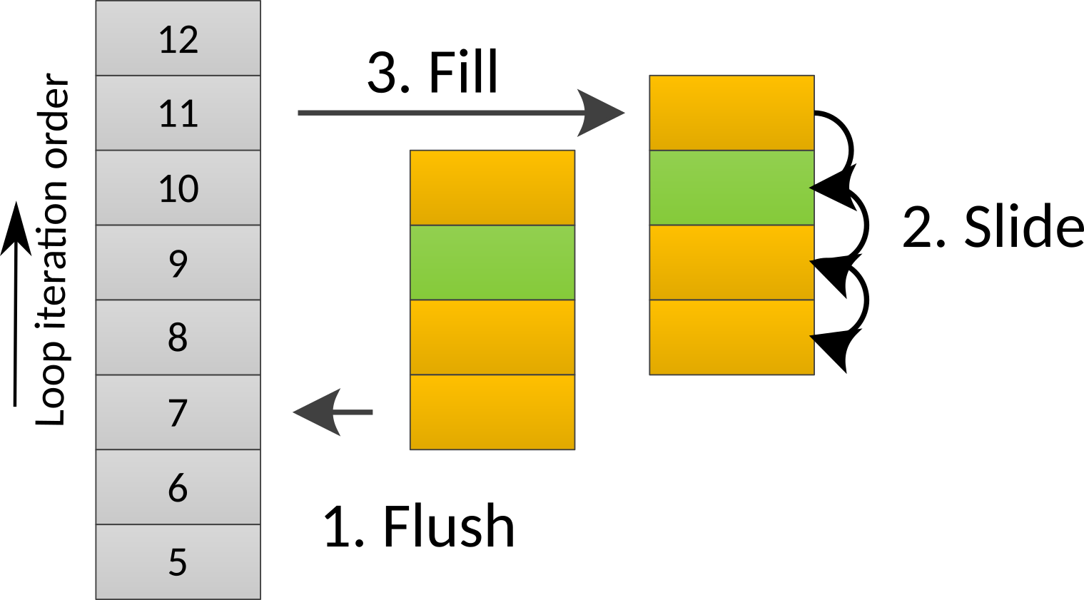
Fig. 3 Representation of an implementation for a cache<cache_type::k, cache_io_policy::fill_and_flush> that is used within a stencil with Extent <-2, 1> in the vertical dimension and implemented as a ring-buffer with 4 levels (in order to allocate all possible offsetted accesses). The three operations are triggered automatically by the library for a fill_and_flush Cache when the vertical loop transition from level 9 to level 10.

Expandable Parameters

Expandable parameters implement a “single stencil multiple storages” pattern. They are useful when we have a vector of storages which have the same shape, and we want to perform the same operation with all of them (a typical situation when implementing e.g. time differentiation schemes). Normally this could be achieved by creating a loop and running multiple computations, but this solution would be inefficient. A more efficient solution is provided through the expandable parameters API.

The user must collect the storages in a std::vector

std::vector<storage_t> list = {
    storage1, storage2, storage3, storage4, storage5, storage6, storage7, storage8};

This std::vector is then used as a storage type with no differences with respect to the regular storages.

The implementation requires the user to specify an integer expand_factor when defining the computation. The optimal value for expand_factor might be backend-dependent.

auto const spec = [](auto s) {
  return execute_parallel().stage(functor(), s);
};
expandable_run<4>(spec, backend_t(), grid, s);

The vector of storages is then partitioned into chunks of expand_factor size (with a remainder). Each chunk is unrolled within a computation, and for each chunk a different computation is instantiated. The remainder elements are then processed one by one.

Summing up, the only differences with respect to the case without expandable parameters are:

• expandable_run has to be used instead of run

• an expand_factor has to be passed to the expandable_run, defining the size of the chunks of

• expandable parameters should be unrolled in each computation.

• a std::vector of storage pointers has to be used instead of a single storage.

All the rest is managed by GridTools, so that the user is not exposed to the complexity of the unrolling, he can reuse the code when the expand factor changes, and he can resize dynamically the expandable parameters vector, for instance by adding or removing elements.

Global Parameters

The API allows the user to define an arbitrary object to act as a Global Parameter as long as it is trivially copyable. To create a Global Parameter from a user-defined object, we pass the object to make_global_parameter()

auto my_global_parameter = make_global_parameter(my_object);

Boundary Conditions

Introduction

The boundary condition module in GridTools is designed following the principle that boundary conditions can be arbitrarily complex, so we want the user to be able to specify any boundary condition code to set up their problems.

Preliminaries

One main concept that is needed for the boundary condition is the one of direction.

In a 3D regular grid, which is where this implementation of the boundary condition library applies, we associate a 3D axis system, and the cell indices (i, j, k) naturally lie on it. With this axis system the concept of “vector” can be defined to indicate distances and directions. Direction is the one thing we need here. Instead of using unitary vectors to indicate directions, as it is usually the case for euclidean spaces, we use vectors whose components are -1, 0, and 1. For example, \((1, 1, 1)\) is the direction indicated by the unit vector \((1, 1, 1)/\sqrt3\). If we take the center of a 3D grid, then we can define 26 different directions \(\{(i, j, k): i, j, k \in \{-1, 0, 1\}\}\setminus\{(0, 0, 0)\}\) that identify the different faces, edges and corners of the cube to which the grid is topologically analogous with.

The main idea is that a boundary condition class specializes operator() on a direction, or a subset of directions, and then perform the user specified computation on the boundaries on those directions.

The user can define their own boundary condition classes and perform specific computation in each direction. For this reason GridTools provides a direction type which can take three direction values, that are indicated as minus_, plus_ and zero_, which are values of an enum called sign.

Boundary Condition Class

The boundary condition class is a regular class which need to be copy constructible, and whose member functions should be decorated with the GT_FUNCTION keyword to enable accelerators. It must not contain references to data that may be not available on the target device where the boundary conditions are applied.

The boundary condition class provides overloads for the operator() which take as first argument a direction object, a number of Data Stores that are the inputs, and three integer values that will contains the coordinate indices of the cell that is being iterated on.

All overloads must have the same number of arguments: the first argument is the direction over which the overload will be applied to, then there is the list of Data Views that will be accessed by the boundary class, and finally three integers that contains the indices of the element being accessed in the call. It is standard practice to let the view types be template arguments. For instance, here a class that applies a copy-boundary condition (copy the second view into the first one) for all direction apart all directions for which the third component is minus_:

struct example_bc {
   double value;

   GT_FUNCTION
   example_bc(double v) : value(v) {}

   template <typename Direction, typename DataField0, typename DataField1>
   GT_FUNCTION void operator()(Direction,
                               DataField0 &data_field0, DataField1 const &data_field1,
                               unsigned i, unsigned j, unsigned k) const
   {
     data_field0(i, j, k) = data_field1(i, j, k);
   }

   template <sign I, sign J, typename DataField0, typename DataField1>
   GT_FUNCTION void operator()(direction<I, J, minus_>,
                               DataField0 &data_field0, DataField1 const &,
                               unsigned i, unsigned j,  unsigned k) const
   {
     data_field0(i, j, k) = value;
   }
};

operator() of the boundary class is called by the library, on the 26 directions, and got each value in the data that correspond to each direction. In the previous example, each direction in which the third component is minus will select the specialized overload, while all other directions select the first implementation.

Boundary Condition Application

To apply the above boundary conditions class to the data fields, we need to construct the boundary object, but also to specify the Halo regions. The Halo regions are specified using Halo Descriptors.

To do this we need an array of Halo Descriptors initialized with the Halo information of the data fields.

Note

The fifth number, namely the total length, in the Halo Descriptor is not used by the boundary condition application module, but kept to reduce the number of similar concepts.

array<halo_descriptor, 3> halos;
halos[0] = halo_descriptor(1, 1, 1, d1 - 2, d1);
halos[1] = halo_descriptor(1, 1, 1, d2 - 2, d2);
halos[2] = halo_descriptor(1, 1, 1, d3 - 2, d3);

After this is done we can apply the boundary condition by, as in this example, constructing the boundary object and applying it to the data fields. The number of data fields to pass is equal to the number of fields the operator() overloads of the boundary class require.

boundary<example_bc, backend_t>(halos, example_bc(42)).apply(out_s, in_s);

As can be noted, the backend is also needed to select the proper implementation of the boundary application algorithm (see Backend). out_s and in_s are the two data fields passed to the application. The fact that the first is the output and second is the input derives from the signature of the overloads of operator(), and it is user defined.

Boundary Predication

Predication is an additional feature to control the boundary application. The predicate type have to be specified as template argument of the boundary class, and the instantiated object of that type passed as third argument of the boundary class constructor, as in the following example:

boundary<direction_bc_input<uint_t>, backend_t, predicate_t>
  (halos, direction_bc_input<uint_t>(42), predicate_t{}).apply(out_s, in_s);

The predicate must obey a fixed interface, that is, it has to accept as argument a direction object, so that the user can, at runtime, disable some operator() overloads. This can be very useful when the user is running on a parallel domain decomposed domain, and only the global boundaries need to updated with the boundary conditions application and the rest should have their Halos updated from neighbors.

Provided Boundary Conditions

GridTools provides few boundary application classes for some common cases. They are

• copy_boundary to copy the boundary of the last field of the argument list of apply into the other ones;

• template <class T> value_boundary to set the boundary to a value for all the data fields provided;

• zero_boundary to set the boundary to the default constructed value type of the data fields (usually a zero) for the input fields.

Halo Exchanges

Introduction

The communication module in GridTools is dubbed GCL. It’s a low level halo-update interface for 3D fields that takes 3D arrays of some types, and the descriptions of the halos, and perform the exchanges in a scalable way.

It is low-level because the requirements from which it was initially designed, required easy interoperability with C and Fortran, so the API takes pointers and sizes. The sizes are specified by halo_descriptor, which are loosely inspired by the BLAS description of dimensions of matrices. A new, more modern set of interfaces are being implemented, to serve more general cases, such as higher dimensions and other grids.

We first start with some preliminaries and then discuss the main interfaces.

Preliminaries

Processor Grid

The processor grid is a concept that describe a 3D lattice of computing elements (you may think of those as MPI tasks). The identifiers of them are tuples of indices. This naturally maps to a 3D decomposition of a data field.

Layout Map

The communication layer needs two Layout Maps: one for describing the data, and one for the processor grid. For the user, the dimensions of the data are always indicated as first, second, and third (or i, j, k), it is the Layout Map that indicates the stride orders, as in the following example:

For instance:

//         i, j, k
layout_map<1, 0, 2>

This Layout Map indicates that the first dimension in the data (i) is the second in the decreasing stride order, while the second (j) has the biggest stride, and last dimension (k) is the one with stride 1. The largest strides are associated to smaller indices, so that layout_map<0, 1, 2> corresponds to a C-layout, while layout_map<2, 1, 0> to a Fortran layout.

The second template Layout Map in the Halo Exchange pattern is the map between data coordinates and the processor grid coordinates.

The following layout specification

layout_map<1, 0, 2>

would mean: The first dimension in data matches with the second dimension of the computing grid, the second dimension of the data to the first of the processing grid, and the third one to the third one. This is rarely different from layout_map<0, 1, 2>, so it can generally be ignored, but we give an example to clarify its meaning.

Suppose the processor grid (domain decomposition sizes) has size PIxPJx1. Now, we want to say that the first dimension on data ‘extends’ to the computing grid on (or that the first dimension in the data corresponds to) the first dimension in the computing grid. Let’s consider a 2x1 process grid, and the first dimension of the data being the rows (i) and the second the column (j). In this case we are assuming a distribution like in Fig. 4.

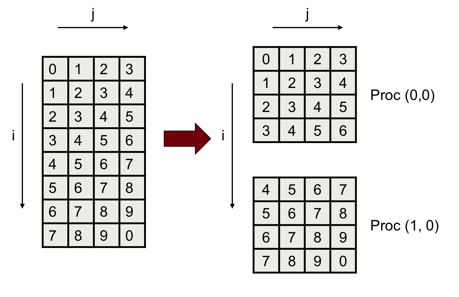
Fig. 4 Example data distribution among two processes.

In this case the map between data and the processor grid is:

layout_map<0, 1, 2> // The 3rd dimension stride is 1

On the other hand, having specified

layout_map<1, 0, 2>

for this map, would imply a layout/distribution like the following Fig. 5.

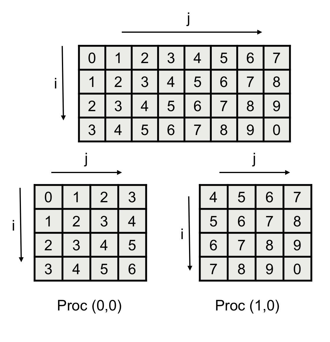
Fig. 5 Example data distribution among two processes.

Where the second dimension in the data correspond to the fist dimension in the processor grid. Again, the data coordinates ordering is the one the user choose to be the logical order in the application, not the increasing stride order.

Halo Descriptor

Given a dimension of the data (array), the communication module requires the user to describe it using the halo_descriptor class, which takes five integers. This class identifies the data that needs to be exchanged.

Consider a dimension which has minus halo lines on one side, and plus halo lines on the other (The minus and plus indicate the sides close to index 0 and the last index of the dimension, respectively). The beginning of the inner region is marked by begin and its ending by end. The end is inclusive, meaning that the index specified by it, is part of the inner region. Another value is necessary, which has to be larger than end - begin + 1 + minus + plus, and is the total_length. This parameter is the equivalent of the “leading dimension” in BLAS. With these five numbers we can describe arbitrary dimensions, with paddings on the left and on the right, such as the example in Fig. 6.

The interface for specifying a halo descriptor is fairly simple, where the name of arguments should be self-explanatory:

halo_descriptor(uint_t minus, uint_t plus, uint_t begin, uint_t end, uint_t total_length)

Todo

annotate example with minus plus begin and end

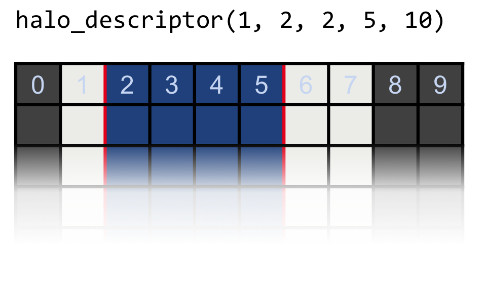
Fig. 6 Example halo descriptor with one halo point on the left and two on the right.

GCL Communication Module

Now we are ready to describe the Halo Exchange patterns objects. The first one is halo_exchange_dynamic_ut. The ut suffix stands for uniform types, meaning that the data fields that this object will manage must all store the same value types, that are declared at instantiation time. The domain decomposition goes up to three dimensions and the data to be exchanged contained in 3 dimensional arrays (lower dimensions can be handled by setting the missing dimensions to 1). Being designed for three dimensional data, the layout maps have three elements (refer to :numref:storage-info for more information).

The type of the object is defined as in this example:

using pattern_type = gcl::halo_exchange_dynamic_ut<layout_map<0, 1, 2>,
                     layout_map<0, 1, 2>, value_type, gcl::cpu>;

The template arguments are:

1. the layout if the data;

2. the mapping between the data dimensions and processing Grid, as described above (leave it as layout_map<0, 1, 2> if in doubt);

3. the type of the values to be exchanged;

4. the place where the data lives and for which the code is optimized. The options for this arguments are gcl::gpu and gcl::cpu.

The Halo Exchange object can be instantiated as:

pattern_type he(pattern_type::grid_type::period_type(true, false, true), CartComm);

Where period_type indicates whether the corresponding dimensions are periodic or not. CartComm is the MPI communicator describing the computing grid.

After the object has been instantiated, the user registers the halos for the corresponding dimension and the five numbers we described above, for the three dimensions (0 is the first dimension).

he.add_halo<0>(minus0, plus0, begin0, end0, len0);
he.add_halo<1>(minus1, plus1, begin1, end1, len1);
he.add_halo<2>(minus2, plus2, begin2, end2, len2);

When the registration is done a setup function must be called before running data exchange. The argument in the set up function is the maximum number of data arrays that the pattern will exchange in a single step. In this example we set it to 3, so that exchanging more than 3 fields will lead to a runtime error. Be aware that setting a larger number of supported fields leads to larger memory allocations. The code looks like:

he.setup(3);

Now we are ready to exchange the data, by passing (up to) three pointers to the data to pack, then calling exchange and then unpack into the destination data, as in the following example:

he.pack(array0, array1, array2);
he.start_exchange();
he.wait();
he.unpack(array0, array1, array2)

Alternatively, the pointers can be put in a std::vector<value_type*> so that the code would look like:

he.pack(vector_of_pointers);
he.start_exchange();
he.wait();
he.unpack(vector_of_pointers);

An alternative pattern supporting different element types is:

using pattern_type = halo_exchange_generic<layout_map<0, 1, 2>, arch_type>;

Now the Layout Map in the type is the mapping of dimensions to the computing grid (the number of dimensions is 3, so the layout map has three elements), and arch_type is either gcl::gpu or gcl::cpu.

The construction of the object is identical to the previous one, but the set-up somewhat more complex now, since we have to indicate the maximum sizes and number of fields we will exchange using this object.

array<halo_descriptor, 3> halo_dsc;
halo_dsc[0] = halo_descriptor(H1, H1, H1, DIM1 + H1 - 1, DIM1 + 2 * H1);
halo_dsc[1] = halo_descriptor(H2, H2, H2, DIM2 + H2 - 1, DIM2 + 2 * H2);
halo_dsc[2] = halo_descriptor(H3, H3, H3, DIM3 + H3 - 1, DIM3 + 2 * H3);

he.setup(4, // maximum number of fields
         field_on_the_fly<int, layoutmap, pattern_type::traits>(null_ptr, halo_dsc),
         sizeof(biggest_type_to_be_used)); // Estimates the sizes

The halo descriptors above indicate the largest arrays the user will exchange, while the field_on_the_fly specify a type and layout (and mandatory traits). The type does not have any effect here, and neither the layout. The traits are important, and the halos are essential. With this pattern, the user needs to indicate what is the size of the largest value type they will exchange.

When using the pattern, each data field should be wrapped into a field_on_the_fly object, such as

field_on_the_fly<value_type1, layoutmap1, pattern_type::traits> field1(
    ptr1, halo_dsc1);
field_on_the_fly<value_type2, layoutmap2, pattern_type::traits> field2(
    ptr2, halo_dsc2);
field_on_the_fly<value_type3, layoutmap3, pattern_type::traits> field3(
    ptr3, halo_dsc3);

Now each field can have different types and layouts, and halo descriptors. The exchange happens very similarly as before:

he.pack(field1, field2, field3);

he.exchange();

he.unpack(field1, field2, field3);

The interface accepting a std::vector also works for this pattern (in case all the fields have the same type).

Distributed Boundary Conditions

Design Principles:

• When doing expandable parameters, the user may want to apply BCs and perform communications on a sub-set of the Data Stores collected in these data representations. For this reason an interface for applying distributed boundary conditions takes single data-stores only.

• The user may want to apply different BCs to the same data-store at different times during an executions, so the binding between BCs and data-stores should be done at member-function level, not at class level, in order to remove the need for instantiation of heavy objects like Halo-updates.

• The same holds for the Data Stores to be exchanged: we need to plug the Data Stores at the last minute before doing the packing/unpacking and boundary apply. The requirement given by the underlying communication layer is that the number of data fields to be exchanged must be less than or equal to the maximum number of data fields specified at construction time.

• The Halo Exchange patterns are quite heavy objects so they have to be constructed and passed around as references. The setup needs to be executed only once to prevent memory leaks.

• The Halo information for communication could be derived by a storage_info class, but there may be cases in which a separate Halo information can be provided, and different storage_info s (with different indices, for instance) may have the same communication requirements (for instance in cases of implicit staggering). For this reason the halo_descriptor is passed explicitly to the distributed boundary construction interface.

• The value_type should be passed as an additional template parameter to the distributed boundaries interfaces. The value_type is used to compute the sizes of the buffers and the data movement operations needed by communication.

Communication Traits

Communication traits helps the distributed boundary condition interface to customize itself to the need of the user. A general communication traits class is available in distributed_boundaries/comm_traits.hpp. The traits required by the distributed boundaries interface, as provided by GridTools, are listed below here.

template <typename StorageType, typename Arch>
struct comm_traits {
  using proc_layout = gridtools::layout_map<...>; // Layout of the processing grid to relate the data layout to the distribution of data
  using proc_grid_type = MPI_3D_process_grid_t; // Type of the computing grid
  using comm_arch_type = Arch; // Architecture for the communication pattern
  compute_arch = backend::...; // Architecture of the stencil/boundary condition backend
  static constexpr int version = gridtools::packing_version::...; // Packing/Unpacking version
  using data_layout = typename StorageType::storage_info_t::layout_t; // Layout of data
  using value_type = typename StorageType::data_t; // Value Type
};

Binding Boundaries and Communication

GridTools provides a facility for applying boundary conditions. The distributed boundaries interfaces uses this facility underneath. The boundary application in GridTools accept specific boundary classes that specify how to deal with boundaries in different directions and predicated to deal with periodicity and domain decomposition. The latter will be dealt by the distributed boundary interfaces (refer to the boundary condition interfaces for more details).

The distributed boundaries interface require a user to specify which Data Stores required communication and which require also boundary conditions, and in the latter case what boundary functions to use.

The way of specifying this is through the function bind_bc which has the following signature:

unspecified_type x = bind_bc(boundary_class, data_stores, ...);

The number of Data Stores is dictated by the boundary_class::operator(), that is user defined (or provided by GridTools).

The Data Stores specified in the function call will be passed to the boundary_class and also used in Halo-update operations.

However, some data fields used in boundary conditions may be read-only and should not be passed to the Halo-update operation, both for avoiding unnecessary operations and to limit the amount of memory used by the Halo-update layer. For this reason the data_store passed the bind_bc can actually be std::placeholders. Only the actual data_store specified in the bind_bc call will be passed to the communication layer. To bind the placeholders to actual data_store the user must bind then using .associate(data_stores...) with the same mechanism used in std::bind as in the following example, in which data_store c is associated to placeholder _1.

using namespace std::placeholders;
bind_bc(copy_boundary{}, b, _1).associate(c)

This example, copies the boundary of c into b, and performs the halo exchanges for b. The halo exchange will not be executed on c, which is read only in this call.

If halo exchanges should be applied to both fields, and the boundary of `c should be copied into b, both fields should be used used in bind_bc:

bind_bc(copy_boundary{}, a, b);

Distributed Boundaries

The distributed boundaries class takes the communication traits as template argument. In the next example we use the communication traits class provided by GridTools, and communication_arch is one of the GCL specifiers of where the data accessed by a Halo Exchange object reside.

using dbs_t = distributed_boundaries<comm_traits<storage_type, communication_arch>>;

During construction more information is required about the Halo structure. We use here the usual Halo Descriptor.

The user needs also to indicate which dimensions are periodic (refer to GCL Communication Module for more information), and this is done using another GridTools facility which is the boollist. Finally, to let the library compute the right amount of memory to allocate before hand, the maximum number of fields to be exchanged in one call have to be specified. The code showing an example of how to do it follows:

halo_descriptor di{halo_sx0, halo_dx0, begin0, end0, len0};
halo_descriptor dj{halo_sx1, halo_dx1, begin1, end1, len1};
halo_descriptor dk{halo_sx2, halo_dx2, begin2, end2, len2};
array<halo_descriptor, 3> halos{di, dj, dk};

boollist<3> periodicity{b0, b1, b2}; // b0, b1, b2 are booleans. If true it will indicate that the corresponding dimension is periodic across the grid of processors.

int max_ds = 4; // maximum number of data stores to be used in a halo_update operation

dbs_t dbs{halos, periodicity, max_ds, MPI_COMMUNICATOR};

Above here the Halo are the local Data Stores sizes, which are usually the tiles of a domain decomposed global domain, which has global boundaries. The idea is to apply the boundary conditions to the global boundaries while performing Halo updates for the Halo regions between sub-domains of the domain decomposed global domain.

The distributed_boundary object allows the user to query the properties of the grid of processes, for instance the coordinates of the current process and the size of the computing grid.

int pi, pj, pk;
dist_boundaries.proc_grid().coords(pi, pj, pk); // Coordinates of current process
int PI, PJ, PK;
dist_boundaries.proc_grid().dims(PI, PJ, PK); // Sizes of the current grid of processes

When invoking the boundary application and Halo-update operations the user calls the exchange member of distributed_boundaries. The arguments of exchange are either Data Stores stores or bind_bc objects which associate a boundary condition to Data Stores. The Data Stores passed directly to the exchange methods have their halo updated according to the halo and periodicity information specified at distributed_boundaries object construction.Arguments created with bind_bc are updated as mentioned above; halo exchanges are only applied if the fields are inside bind_bc, but not in associate.

Next, we show a complete example where two boundary are applied using a fixed value on Data Store a and a copy_boundary to copy the value of Data Store c into Data Store b (refer to GCL Communication Module). The halos of data store c will not be exchange; this field serves as source of data for the copy_boundary. Three fields will have their Halo updated by the next example, namely a, b and d:

dist_boundaries.exchange(bind_bc(value_boundary<double>{3.14}, a), bind_bc(copy_boundary{}, b, _1).associate(c), d);

An additional facility provided is an alternative to the exchange method. This is used to skip the Halo updates altogether, and it is called boundary_only, and the code to use it is identical to the previous example, barring the function name:

dist_boundaries.boundary_only(bind_bc(value_boundary<double>{3.14}, a), bind_bc(copy_boundary{}, b, _1).associate(c), d);

This function will not do any halo exchange, but only update the boundaries of a and b. Passing d is possible, but redundant as no boundary is given.

Interfacing to other programming languages

GridTools provides an easy macro interface to generate bindings to C and Fortran. This library is available separately at GridTools/cpp_bindgen.

To make the cpp_bindgen library available the recommended way is to use CMake’s FetchContent as follows

include(FetchContent)
FetchContent_Declare(
  cpp_bindgen
  GIT_REPOSITORY https://github.com/GridTools/cpp_bindgen.git
  GIT_TAG        master # consider replacing master by a tagged version
)
FetchContent_MakeAvailable(cpp_bindgen)

Suppose, the user wants to export the function add_impl.

int add_impl(int l, int r) {
    return l + r;
}

The macros BINDGEN_EXPORT_* provide ways to generate bindings to functions. The different flavours of this macro are explained below. The macro generates a wrapper around the function add_impl which is called add and registers the function to be exported.

#include <cpp_bindgen/export.hpp>
BINDGEN_EXPORT_BINDING_2(add, add_impl);

The user can generate a C header and a Fortran module that matches this header by adding a call to bindgen_add_library in his CMake project:

bindgen_add_library(add_lib SOURCES add.cpp)

This will generate a library add_lib which contains the exported symbol add, and it will generate a target add_lib_declarations that generates the files add_lib.h and add_lib.f90 containing the bindings that can be used from C and Fortran.

The C header contains the exported function (boilerplate code removed):

int add(int, int);

The generated Fortran module contains the corresponding declaration:

module add_lib
implicit none
  interface
    integer(c_int) function add(arg0, arg1) bind(c)
      use iso_c_binding
      integer(c_int), value :: arg0
      integer(c_int), value :: arg1
    end function
  end interface
end

Exporting functions with no array-type arguments

There exist various flavours of these macros. Functions which are non-templated or fully-specialized can be exported with BINDGEN_EXPORT_BINDING, for example:

int add_impl(int, int) { return 0; }
BINDGEN_EXPORT_BINDING_2(add, add_impl);

template <typename T>
T add_impl(T, T) { return {}; }
BINDGEN_EXPORT_BINDING(2, add_impl<int, int>);

All functions exist in two flavours: Either you can pass the number of arguments as part of the name of the macro (BINDGEN_EXPORT_BINDING_2 stands for two arguments), or you can pass it as a first argument to the generic BINDGEN_EXPORT_BINDING. The first flavours exist for up to 9 arguments.

Note that BINDGEN_EXPORT_BINDING_X requires a name and a function pointer as its arguments. A lambda cannot be passed as function pointer; thus, the type of the arguments cannot be deduced. In such cases, the functions can be exported with BINDGEN_EXPORT_BINDING_WITH_SIGNATURE_X, which additionally takes the function type as an argument:

BINDGEN_EXPORT_BINDING_WITH_SIGNATURE_2(add, int(int, int), [](int l, int r) { return l + r; });

Templated functions can be exported for a given set of specializations using BINDGEN_EXPORT_GENERIC_BINDING_X. In addition to the function name and the function pointer, it takes a list of overloads for which the bindings are generated:

BINDGEN_EXPORT_GENERIC_BINDING(2, add, add_impl, (int, int)(double, int));

In the generated Fortran module, generic bindings will produce an interface combining the different overloads:

interface
  integer(c_int) function add_f0(arg0, arg1) bind(c)
    use iso_c_binding
    integer(c_int), value :: arg0
    integer(c_int), value :: arg1
  end function
  real(c_double) function add_f1(arg0, arg1) bind(c)
    use iso_c_binding
    real(c_double), value :: arg0
    integer(c_int), value :: arg1
  end function
end interface
interface add
  procedure add_f0, add_f1
end interface

Complex types

Only a limited set of types can be passed from Fortran / C through the C bindings interface to C++, namely integral and floating point types, booleans and pointers to those types.

Array references, GridTools storages, and any type that is fortran_array_bindable appear as bindgen_fortran_array_descriptor in the C bindings. This structure allows the user to describe the data that needs to be passed to C++.

It is possible to write bindings to functions that accept or return other types. During the generation process, they are replaced with pointers to the type bindgen_handle.

std::vector<int> make_vector_impl() { return {}; }
void use_vector_impl(std::vector<int>) {}
BINDGEN_EXPORT_BINDING_0(make_vector, make_vector_impl);
BINDGEN_EXPORT_BINDING_1(use_vector, use_vector_impl);

The code above will generate the following signatures in the C-header:

bindgen_handle* make_vector();
void use_vector(bindgen_handle*);

The user needs to make sure that the types that stand behind bindgen_handle match, otherwise an exception will be thrown.

Exporting functions with array-type arguments to Fortran

Special macros exist to export function that take array-like arguments to Fortran. While the normal macros export such arguments as bindgen_fortran_array_descriptor, the “wrapped” macros create additional wrappers around the functions that fill the structures themselves.

void dummy_impl(int (&a)[2][2]) {}
BINDGEN_EXPORT_BINDING_WRAPPED_1(dummy, dummy_impl);

The function dummy_impl is taking a reference to an array. When exporting this function with BINDGEN_EXPORT_BINDING_WRAPPED_X, an additional wrapper is generated in the Fortran bindings:

module add_lib
implicit none
  interface
    subroutine dummy_impl(arg0) bind(c, name="dummy")
      use iso_c_binding
      use array_descriptor
      type(bindgen_fortran_array_descriptor) :: arg0
    end subroutine
  end interface
contains
    subroutine dummy(arg0)
      use iso_c_binding
      use array_descriptor
      integer(c_int), dimension(:,:), target :: arg0
      type(bindgen_fortran_array_descriptor) :: descriptor0

      descriptor0%rank = 2
      descriptor0%type = 1
      descriptor0%dims = reshape(shape(arg0), &
        shape(descriptor0%dims), (/0/))
      descriptor0%data = c_loc(arg0(lbound(arg0, 1),lbound(arg0, 2)))

      call dummy_impl(descriptor0)
    end subroutine
end

This allows to call the Fortran function dummy in a convenient way:

integer(c_int), dimension(:, :) :: some_array
call dummy(some_array)

The bindings will take care that the rank matches and it will infer the size of the array automatically.

All additional macros behave as mentioned above, namely BINDGEN_EXPORT_BINDING_WITH_SIGNATURE_WRAPPED, and BINDGEN_EXPORT_BINDING_GENERIC_WRAPPED.

Data types need to be fortran_array_wrappable in order to be compatible with these macros. Natively, only C arrays and fortran_array_adapter are fortran_array_wrappable. The latter is an adapter between Fortran arrays and GridTools storages, such that the user can pass a Fortran array to a C++ function, which then can be transformed into a GridTools storage.

#include <gridtools/storage/adapter/fortran_array_adapter.hpp>

using storage_info_t = storage_traits<Backend>::storage_info_t<0, 3>;
using data_store_t = storage_traits<Backend>::data_store_t<double, storage_info_t>;

void modify_array_impl(fortran_array_adapter<data_store_t> inout) {
    data_store_t data_store{storage_info_t{10, 10, 10}};
    transform(data_store, inout);

    // use data_store

    transform(inout, data_store);
}
BINDGEN_EXPORT_BINDING_WRAPPED_1(modify_array, modify_array_impl)

CMake usage

A call to bindgen_add_library generates the libraries and the headers. By default, the C header file and the Fortran file is written directly into the source tree. This choice was taken to improve building in cross-build environments, because the process cannot rely on generated binaries being executable on the host system. The output folder can be overwritten by setting FORTRAN_OUTPUT_DIR and C_OUTPUT_DIR.

By default, the name of the generated Fortran module is set to the name of the library. A different name can be set with FORTRAN_MODULE_NAME.