Internal Documentation

Indexing Algorithm (Pointer Offset Computation)

On the GridTools frontend side we are using storage_info, data_store and data_view objects when we deal with data. Once this information is passed to the aggregator_type and the intermediate the information how to access the different fields is extracted. This means we extract the raw pointers to the data from the data_store objects and the stride information is from the storage_info objects. The pointers and the strides information are stored in the iterate_domain. In order to save registers and not wasting resources different storage_info instances with a matching ID parameter are treated as a single instance. This can be done because the contained stride information has to be the same if the ID is equal. Fig. 7 shows the storage flow from the frontend to the backend. In this example three data stores are created by the user, and two temporaries are created in the intermediate. The intermediate is extracting the needed information from the data_store and storage_info objects and is feeding the backend with raw data pointers and stride information.

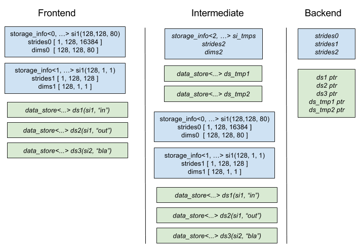
Fig. 7 Transformations applied to storages while passing from frontend to backend.

Old Indexing Approach

As seen before the backend contains stride information and raw data pointers. Unfortunately this is not enough. The backend additionally has to store an offset (called index). The reason for this is that the compute domain is split up into several blocks. Each block is passed to a GPU streaming multiprocessor that contains several cores. Each core has to know its position within the block in order to compute at the right point. So additionally to the stride and pointer information that is shared per block an index is stored per core. Fig. 8 shows the contents of two independent blocks. As visible the stride and pointer information is the same but the index is different for each thread.

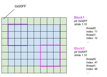
Fig. 8 Old GridTools indexing approach.

The index is computed as follows. If there is no Halo the index will be

\[\begin{split}\begin{align} i &= (block\_id\_x * block\_size\_x + thread\_id\_x) * stride\_i \\\\ &+ (block\_id\_y * block\_size\_y + thread\_id\_y) * stride\_j \end{align}\end{split}\]

In case of a Halo the index is shifted into the right direction (like visible in Fig. 8).

Issues Regarding Temporaries

Temporary storages share the same storage_info because they all have the same size. The problem with temporaries is that computations in the Halo region have to be redundant because we don’t know when the data will be available. To solve the problem with redundant computations the temporary storages, that are allocated in the intermediate, are extended by a certain number of elements. The size of the CUDA block is known beforehand and also the size of the Halo and the number of blocks/threads is known. With this information an extended temporary storage can be instantiated. For performance reasons we want the first non-Halo data point of each block to be in an aligned memory position. Therefore we add a certain number of padding elements between the blocks. Fig. 9 compares the non-aligned versus the aligned storages. The green dots are marking the Halo points. It can be seen that each block has its own Halo region. The blue squares are padding elements and the yellow squares are data points. As visible on the right part of the drawing the first data point should be in an aligned memory position. In order to achieve this padding elements are added between the blocks.

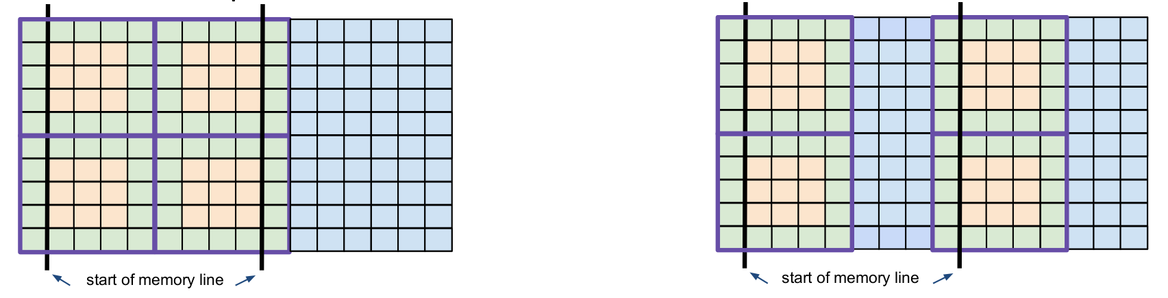
Fig. 9 Alignment issues on temporary storages.

Base Pointer Change

When the aligned temporary improvement was introduced the logic in the backend was slightly changed. As shown before the backend contains a pointer to each of the storage. In combination with an index the cuda thread can identify its compute position. When temporaries are used one cannot just simply use a base pointer for all the cuda blocks and just multiply the current block index with the block size like shown in the formula above. The base pointer has to be computed per block. So each block contains a pointer to its own temporary storage. See Fig. 10.

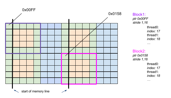
Fig. 10 Per-block private base pointers.

There is no difference in resource consumption when using the changed base pointer approach. It was mainly introduced for convenience and in order to smoothly integrate the aligned temporary block improvement.

Multiple Temporaries with Different Halo

Formerly GridTools used one storage_info per temporary storage. This is convenient but consumes more resources than needed. Therefore it was replaced by the more resource efficient "one storage_info for all temporaries" solution. The temporaries are all having the same size. So the stride information can be shared in the backend. The only problem occurs when different temporaries (with the same size, as mentioned before) are accessing different Halos. The base pointer is set correctly only for the temporary that is using the maximum Halo. All the other temporaries are unaligned by $max_halo - used_halo$ points. This happens for instance when computing the horizontal diffusion. The flx and fly temporaries use different Halos. In this case the temporary written in the flx stage will be properly aligned because it is accessing the maximum Halo in the aligned direction (x direction). The second temporary written in the fly stage will be unaligned because it does not use the Halo points in x-direction. In order to fix this alignment mistake the missing offset is added when setting the base pointer. The information that is passed to the algorithm that extracts the base pointer knows about the used Halo of each storage and also the maximum Halo in the alinged direction. A value of $max_halo - used_halo$ is added to each base pointer.

Passing Huge Types Down to the Offset Computation

In order to fix the alignment when using different Halos we have to pass a lot of type information from the intermediate down to the backend. This is exhaustive for the compiler and the performance suffers. This could lead to problems, especially when trying to compile computations with many stages and a high number of fields.

Updated Indexing Algorithm

The new indexing approach tries to avoid the strategy of setting the base pointer to the first point of the block. The new approach is to set the pointer to the first non-Halo point of the block. The method that is setting the index of each cuda thread has to be modified. Fig. 11 shows the new indexing. As shown, the first non Halo point is used as base pointer. The index is also modified in order to point to the correct data location.

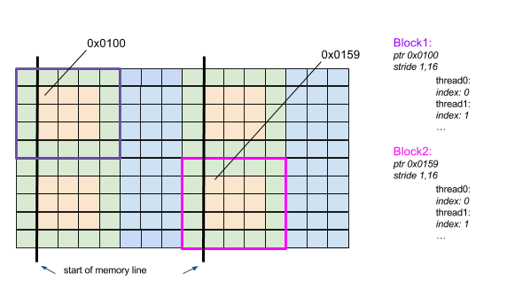
Fig. 11 Per-block private base pointers to first non-Halo point of the block.

Data Dependence Analysis in GridTools

(copied from the wiki)

A multistage stencil is a sequence of stages. Each stage is (basically) made of a stencil operator and a list of placeholders. Each placeholders is associated to the arguments in the param_list of the stencil operator positionally, that is, as it would happen if the placeholders were passed to the stencil operator according to the param_list. The param_list lists accessors, and each accessor have an extent. Each accessor has also an intent, which represents the use the stencil operator is going to make of the data, either read-only or read-write.

So, given a stage we can associate to each placeholder an extent and an intent, simply by scanning the accessors in the param_list of the stage.

Consider the last stage in a multistage computation. This will have one (or more) output accessors in the param_list of the stencil operator, so one (or more) placeholders in the list. This output will be computed by accessing the inputs within the extents that are specified in the corresponding accessors. Now, let’s move to the stage just before that. Some of its inputs may be used by the last stage as inputs. This means that those outputs must be computed in a set of points that will be consumed by the next stage.

A very simple example

Let us consider an example (in 1D for simplicity). Suppose we have the following concatenation of stages, where we write at the left the outputs and on the right, with an associated extent, are the inputs:

a <- f0(b<-1,1>, c<0,1>)
d <- f1(b<-2,0>, c<-1,2>)
e <- f2(a<-1,2>, d<-2,2>, c<-1,1>)

We call the arguments placeholders, to be closer to the GridTools algorithm. We have 5 placeholders and we start with an initial map such as:

a -> <0,0>
b -> <0,0>
c -> <0,0>
d -> <0,0>
e -> <0,0>

Now we visit our sequence of stages from the last to the first. The last computes e and then needs a, d, and c in different extents. We update the map as follow:

a -> <-1,2>
b -> <0,0>
c -> <-1,1>
d -> <-2,2>
e -> <0,0>

Next we examine f1. It writes d, and since d is needed in an interval <-2,2> by f2, we need to update it’s inputs that need now to be read at an extent that is <-2,2> + <x,y>, where <x,y> is the extent of an input and the + operation corresponds to the following operation: <x,y> + <u,v> = <x+u, y+v>. If the extent needed for the inputs are smaller than the one contained in the map already, we do not update the map, since the needed values are already there. We do it by using the mee function that returns the minimum enclosing extent of two extents. So now we update the map as follow:

a -> <-1,2>
b -> mee(<0,0>, <-2,2>+<-2,0>) = <-4,2>
c -> mee(<-1,1>, <-2,2>+<-1,2>) = <-3,4>
d -> <-2,2>
e -> <0,0>

Now to the last stage to examine: f0. It writes a and needs b<-1,2> and c<0,1>. According the the map, a is needed in <-1,2> so

a -> <-1,2>
b -> mee(<-4,2>, <-1,2>+<-1,1>) = mee(<-4,2>, <-2,3>) = <-4,3>
c -> mee(<-3,4>, <-1,2>+<0,1>) = mee(<-3,4>, <-1,3>) = <-3,4>
d -> <-2,2>
e -> <0,0>

The fields a and d are written and the read. They are eligible to be temporary fields. b and c are inputs, and they are needed in <-4,3> and <-3,4> respectively. So the number of “halos” around them should be appropriate to avoid access violations. The field e is the output and it’s written in a single point.

If we compute f2 in a point, we need to compute f1 in <-2,2>, since this will produce the values needed by f2. We then need to compute f0 in <-1,2> to produce the values needed for a.

A more complex example

The next example is very similar to the previous one, but now the second stage uses a instead of c.

a <- f0(b<-1,1>, c<0,1>)
d <- f1(b<-2,0>, a<-1,2>)
e <- f2(a<-1,2>, d<-2,2>, c<-1,1>)

The map, then, after examining f2 is as before

a -> <-1,2>
b -> <0,0>
c -> <-1,1>
d -> <-2,2>
e -> <0,0>

When we examine f1, however, the extents become:

a -> mee(<-1,2>, <-2,2>+<-1,2>) = <-3,4>
b -> mee(<0,0>, <-2,2>+<-2,0>) = <-4,2>
c -> <-1,1>
d -> <-2,2>
e -> <0,0>

When we move to f0:

a -> <-3,4>
b -> mee(<-4,2>, <-3,4>+<-1,1>) = <-4,5>
c -> mee(<-1,1>, <-3,4>+<0,1>) = <-3,5>
d -> <-2,2>
e -> <0,0>

So, now, to compute f2 in a point we need to compute f1 in <-2,2> and f0 in <-3,4>. Note that, when f2 access a in <-1, 2>, those values have been computed in abundance to allow the computation of f1.

Catching bad dependencies

Let’s consider another variation on the same example. Now f1 writes into c, and d becomes an input.

a <- f0(b<-1,1>, c<0,1>)
c <- f1(b<-2,0>, a<-1,2>)
e <- f2(a<-1,2>, d<-2,2>, c<-1,1>)

As before the map after examining f2 is

a -> <-1,2>
b -> <0,0>
c -> <-1,1>
d -> <-2,2>
e -> <0,0>

When we analyze f1 we have

a -> mee(<-1,2>, <-1,1>+<-1,2>) = <-2,3>
b -> mee(<0,0>, <-1,1>+<-2,0>) = <-3,1>
c -> <-1,1>
d -> <-2,2>
e -> <0,0>

And then f0

a -> <-2,3>
b -> mee(<-3,1>, <-2,3>+<-1,1>) = <-3,4>
c -> mee(<-1,1>, <-2,3>+<0,1>) = <-2,4>
d -> <-2,2>
e -> <0,0>

But now we have a problem, if we apply the previous strateg. f1 is computed to compute c in <-2,4>, the extent associated by the map. A next element of the output would then read the modified values of c and this is probably wrong. We need to catch this as a problem. We cannot write into a field that is accessed in an extent different than <0,0> in a previous stage. We need a check for this, but it is not yet implemented.

Design of Grid Topology for Irregular Grids

The GridTopology concept provides:

1. Connectivity information to neighbours in the same and different LocationType’s.

2. Storage maker functionality

The icosahedral grid class requires a class, as a template parameter, that implements a GridTopology

template <typename Axis, typename GridTopology>
struct grid

and can be constructed additionally with a runtime instance of the GridTopology, depending on whether the concrete implementation of that GridTopology requires runtime connectivity information.

Currently there are two concrete implementations of the GridTopology:

1. The icosahedral_topology provides connectivity information at compile time, for icosahedral/octahedral grid layouts where all the connectivity information can be derived at compiled time from the parallelogram structures based on simple stride rules.

An example of such structured index layout of the icosahedral grid parallelograms is shown in Fig. 12, where the parallelogram can be indexed with three coordinates i and j and a color that identifies downward/upward triangles. This particular data layout assumes an order in the dimensions like i-c-j (being i the stride - 1 dimension). As an example, the cell with index 14, can be accessed with {i, c, j} coordinates {2, 0, 1}. A similar scheme of indexing for edges, and vertices is developed. All neighbour indexes of any cell/edge/vertex as well as connectivity to different LocationType can be express with simple offset rules.

For example, the neighbor indices of any cell can be computed with the following rules:

{{i - 1, c - 1, j}, {i, c - 1, j + 1}, {i, c - 1, j}} for downward triangle (color==1)
{{i, c + 1, j}, {i + 1, c + 1, j}, {i, c + 1, j - 1}} for upward triangle

Similar rules are derived for connectivities among different location types.

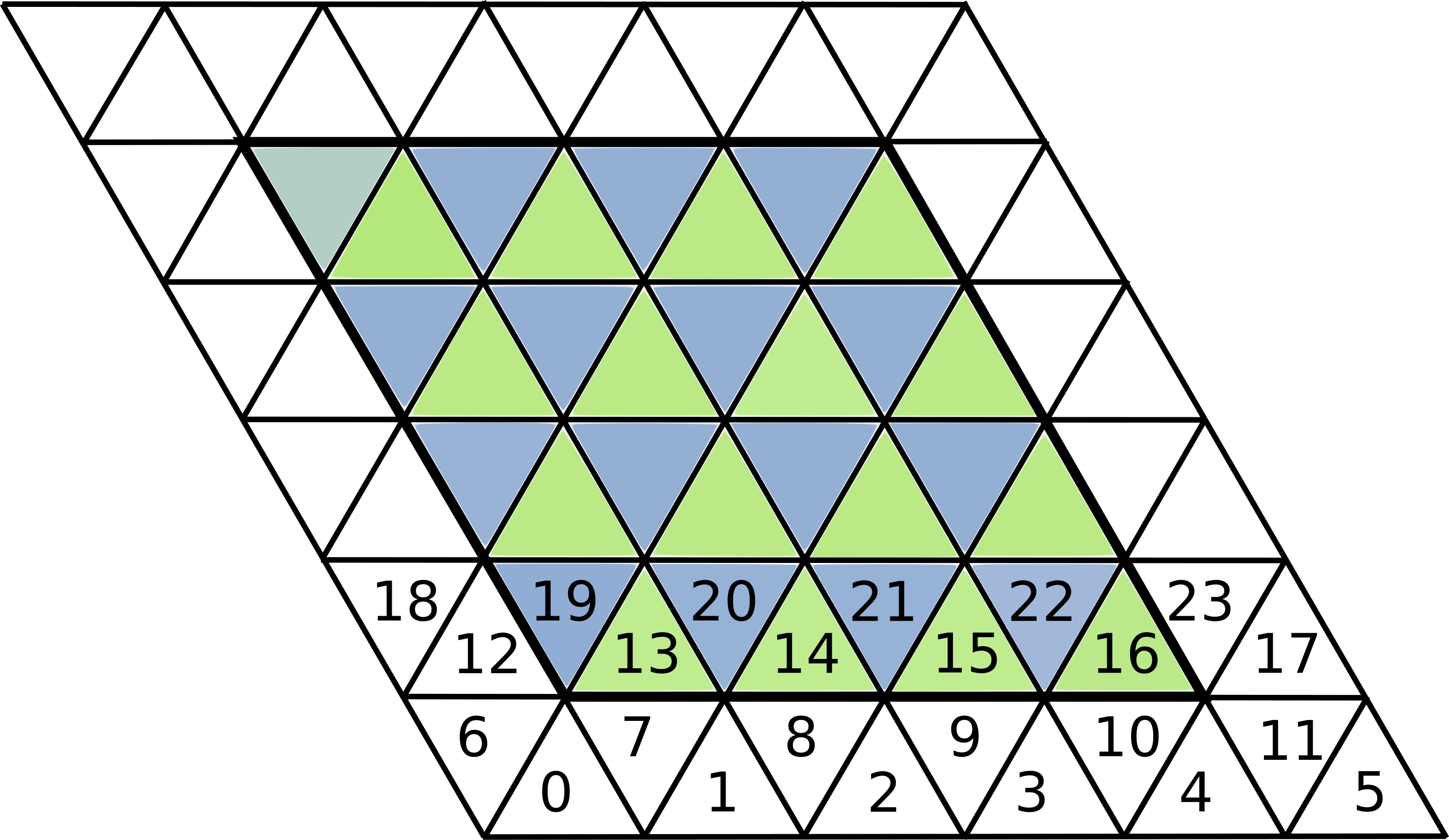
Fig. 12 Structured index layout for icosahedral grid

Since all offset rules are based on the structured of the icosahedral parallelograms, and do not depend on a particular runtime instance of the grid topology, they are derived at compile time. These offsets rules can be extracted using the connectivity class API

template <typename SrcLocation, typename DestLocation, uint_t Color>
struct connectivity

For the icosahedral grid, the connectivity tables give access to the following 9 type of queries, depending on the from and to location types. See Fig. 13.

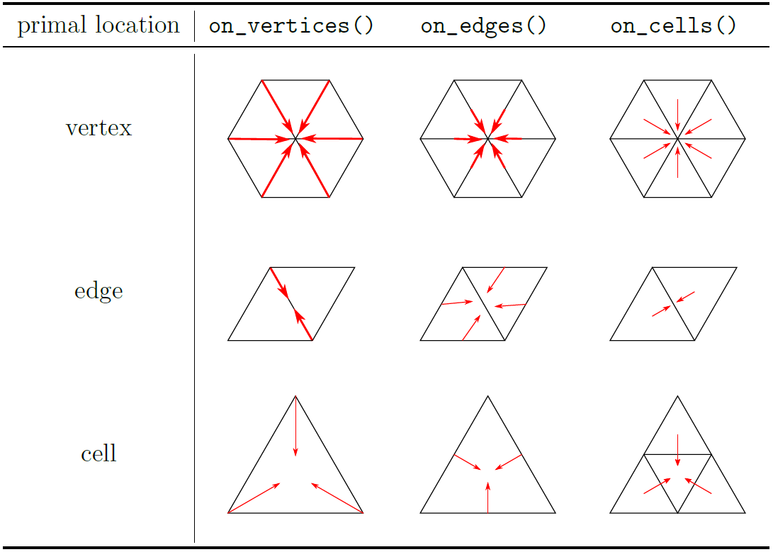
Fig. 13 All possible connectivity queries in an icosahedral grid.

Note

Depending on the location type, there are different number of neighbour indices. For example from<cell>::to<edge> will return a tuple of three edge indices. The order of those neighbours, is part of the API and is defined based on physical meaning of PDE operators.

2. The unstructured_mesh implements a GridTopology for grid layouts without a clear structure, and therefore runtime lookup tables need to be used in order to define connectivities between the different LocationTypes.

Since the connectivity information is stored as lookup tables, the unstructured_mesh needs to accept in the ctr an Atlas mesh object, that contains all the necessary lookup tables. All 9 lookup tables are then stored in two type of (atlas data structure) tables: MultiBlockConnectivity and IrregularConnectivity. The main difference is that the connectivity described with a MultiBlockConnectivity shows a uniform number of neighbours for each entry in the table, while in the IrregularConnectivity, each entry can have a different number of neighbours.

Unstructured Mesh

The grid concept has a GridTopology type, that can be of two classes (as described above). Additionally for the types of GridTopology that require a runtime information with the connectivity tables, the grid also has an unstructured mesh instance of type

using unstructured_mesh_t =
  typename boost::mpl::if_c<is_unstructured_mesh<GridTopology>::value, GridTopology, empty>::type;

In case of having a GridTopology of icosahedral_topology the instance that gets instantiated is an empty class.

Later this unstructured_mesh will be passed to the iterate_domain that requires the connectivity information.

Splitters

Introduction

This document introduces a prototype code used for the development of a new stencil library. The prototype is based on an interval concept, which allows the library user to split an axis of the stencil application domain into arbitrary intervals. Using these intervals it shall be possible to define interval specific stencil update functions. The prototype uses splitters in order to sub-divide an axis. Splitters are ordered positions defined at compile-time. Note that splitters only define an order but not yet an absolute position. At runtime the splitters are placed at an absolute position, in between two axis positions. Due to this staggered placement it is easier to define loop direction independent intervals. Given the splitters we define levels, which specify a position at an offset relative to a splitter. The offset is a small positive or negative integral value limited by a predefined maximum, e.g. 3. The zero offset is undefined as the splitters are not placed in between two axis positions. Given two levels we define closed intervals, which specify a loop direction independent range on the axis. See Figure 1 for an example interval definition. Note that intervals are always defined in axis direction, meaning the “from level” is placed before the “to level” in axis direction.

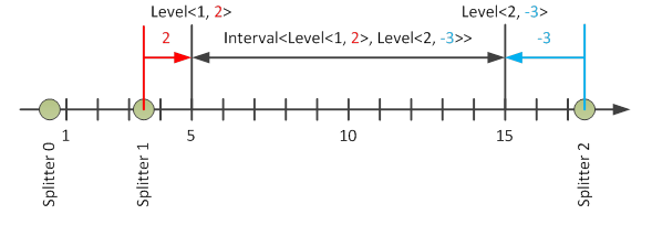
Fig. 14 Splitters, levels and intervals

Figure 1 shows an axis divided by three splitters and an interval spanning the range [5, 15]. Note that there are N * (N-1) / 2 intervals with N being the total number of levels. In order to simplify the implementation the prototype internally represents all levels using a unique integer index. Given a level (splitter and offset) we can compute an index as splitter times number of offsets per splitter plus offset index. The offset index is defined by a mapping of the offset values in a positive and continuous range, i.e. the offsets [-2, -1, 1, 2] are mapped to the offset indexes [0, 1, 2, 3]. Given an index we can compute a level by dividing the index by the number of offsets per splitter. The result corresponds to the level splitter while the remainder corresponds to the offset index which can be mapped back to a level offset.

Note that the FunctorDoMethods.cpp for test purposes converts an integer range into levels and back into indexes resulting in the following output:

Index: 0        Level(0, -3)
Index: 1        Level(0, -2)
Index: 2        Level(0, -1)
Index: 3        Level(0, 1)
Index: 4        Level(0, 2)
Index: 5        Level(0, 3)
Index: 6        Level(1, -3)
Index: 7        Level(1, -2)
Index: 8        Level(1, -1)
Index: 9        Level(1, 1)
Index: 10       Level(1, 2)
Index: 11       Level(1, 3)
Index: 12       Level(2, -3)
Index: 13       Level(2, -2)
Index: 14       Level(2, -1)
Index: 15       Level(2, 1)
Index: 16       Level(2, 2)
Index: 17       Level(2, 3)
Index: 18       Level(3, -3)
Index: 19       Level(3, -2)

Interval Specific Do Methods

The stencil library user will define its update functions using functor objects with interval specific Do methods. The Do method overloads allow defining an interval specific update function for certain sub domains:

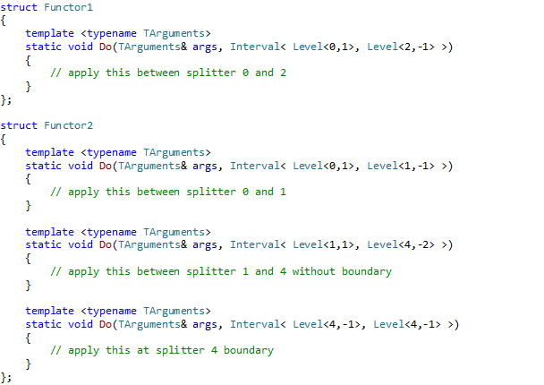
Fig. 15 Functors with interval specific Do method overloads

Note that the functors in the listing define Do method overloads for boundary levels as well as for larger axis sub domains. In order to avoid inconsistencies we define the following rules: - The Do method intervals shall not overlap - The Do method intervals shall be continuous, i.e. gaps are not allowed As the Do method overloads are continuous we can use them in order to compute the loop bounds. Essentially we want to loop from the first Do method interval “from level” to the last Do method interval “to level”.

Loop Interval Computation

Given one or more functors the loop interval computation prepares the stencil library loop execution. Figure 2 illustrates the loop interval computation algorithm, which computes a list of maximal size loop intervals such that there is a unique set of Do method overloads per loop interval. Using these loop intervals the actual loop execution is a simple iteration over all intervals, executing a nested loop over all functors for each interval. Thanks to the loop interval definition we can work with the same set of Do method overloads on the full loop interval.

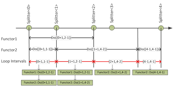
Fig. 16 Loop interval computation algorithm (Do method overloads in black; computed loop intervals in red)

Note that the algorithm assumes that it is possible to query all Do method overloads of a functor. The loop interval computation performs the following steps: 1. Compute a Do method overload list for each functor 2. Compute a loop interval list using the functor Do method lists 3. Compute a vector of functor Do method overload pairs for every loop interval

Do Method Overloads

In order to compute a list of all functor Do method overloads, we iterate over all intervals and store the ones which have a corresponding functor Do method overload. Additionally we can check if the functor follows our rules, i.e. the intervals do not overlap. The Do method overload algorithm works on the following inputs: - Functor – Functor object - Axis – Maximal interval used for the Do method overload search The following pseudo code implements the Do method overload algorithm:

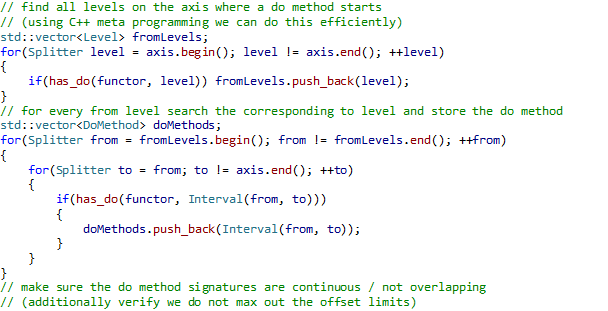
Fig. 17 Functor Do method overload algorithm

Searching all possible Do method intervals has complexity O(N2). Unfortunately we had to abandon this idea due to long compilation times. Therefore we introduced a hack which allows speeding up the search. It is based on the fact that the has_do implementation finds all Do methods of a functor which are callable taking overload resolution into account. Therefore we added a conversion constructor on the interval class which converts a from level into an interval. Due to this implicit conversion we can search for any interval starting at a given from level, using the existing has_do implementation. The only drawback is a nasty error message in case a functor defines multiple Do methods which start at the same from level. Currently we are not aware of a way to catch the error inside the library. In addition to the algorithm presented above the prototype introduces a number of checks. For instance Do methods are not allowed to start or end at the maximum or minimum offset values around a splitter. This boundary of unoccupied levels is used for the loop interval computation, i.e. the loop interval computation has to introduce new levels right before and after the Do methods. The other checks make sure the code complies with our rules that the Do method overloads shall be continuous. The following input-output pairs illustrate the algorithm:

• Functor1, Axis([0,-3],[4,+3]) -> Interval([0,1],[2,-1])

• Functor2, Axis([0,-3],[4,-2]) -> Interval([0,1],[1,-1]), Interval([1,1],[4,-2])

• Functor2, Axis([4,-1],[ 4,-1]) -> Interval([4,-1],[ 4,-1])

## Loop Intervals The loop interval computation overlays all functor Do method intervals and splits them up into loop intervals. Every loop interval is a sub interval of exactly one functor Do method interval. For an illustration have a look at the red loop intervals in Figure 2. The loop interval computation works on the following inputs: - DoMethods – Vector containing a Do method vector for every functor - Axis – Maximal interval used for the Do method overload search The following pseudo code implements the loop interval computation algorithm:

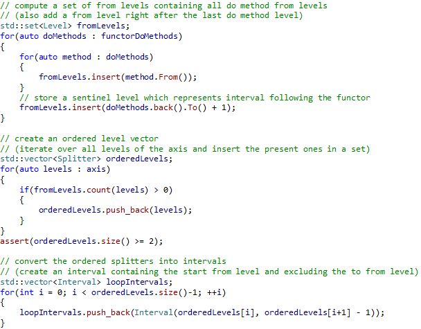
Fig. 18 Loop interval algorithm

The above algorithm uses a set instead of a sorted collection in order to store the relevant levels. Once the set is complete we convert it to a sorted collection via ordered iteration over all levels of the axis. Note that we work with the index level representation which allows us to easily go to the next or previous level using addition respectively subtraction. These operations are ok as we are sure our Do method from and to levels are not splitter boundary levels. It is important to introduce a sentinel level after the last Do method interval in order to properly compute the loop interval for the last Do method interval of a functor. Apart from that the loop interval computation is very smooth and there are no special cases to consider.

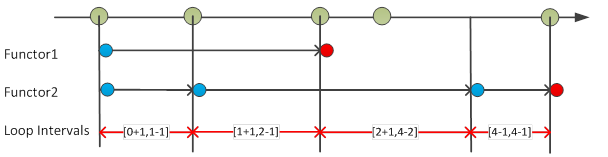
Fig. 19 Loop interval computation (note the read sentinel levels after the last functor do method)

Do Method Lookup Map

The Do method lookup map computation creates a map which associates to every loop interval the matching Do method interval of a functor. We compute such a map for every functor, which later on helps us to compute on-the-fly the matching Do method overloads given a loop interval. The Do method lookup map computation works on the following inputs: - DoMethods – Do method vector containing all Do methods of a functor - LoopIntervals – List containing all loop intervals The following pseudo code implements the Do method lookup map computation:

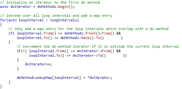
Fig. 20 Do method lookup map algorithm

The algorithm iterates over loop intervals and Do method intervals at the same time, creating a mapping between loop intervals and Do method intervals. Usually the Do method intervals span a larger domain than the loop intervals. Therefore the mapping is not 1:1.

Prototype

The interval prototype code implements the algorithms discussed in chapter 3. The main logic is implemented by the following three files:

• FunctorDoMethods.h

• LoopIntervals.h

• FunctorDoMethodLookupMaps.h

For every file there is a separate test program, while the main.cpp runs the full algorithm. Using boost for_each the test code iterates over all loop intervals and calls the matching functor do method overloads:

Run Functor0, Functor1 and Functor2:
        -> Loop (0,1) - (1,-1)
                -> Functor1:Do(Interval<Level<0,1>, Level<2,-1> >) called
                -> Functor2:Do(Interval<Level<0,1>, Level<1,-1> >) called
        -> Loop (1,1) - (2,-1)
                -> Functor1:Do(Interval<Level<0,1>, Level<2,-1> >) called
                -> Functor2:Do(Interval<Level<1,1>, Level<3,-1> >) called
        -> Loop (2,1) - (3,-2)
                -> Functor2:Do(Interval<Level<1,1>, Level<3,-1> >) called
        -> Loop (3,-1) - (3,-1)
                -> Functor0:Do(Interval<Level<3,-1>, Level<3,-1> >) called
                -> Functor2:Do(Interval<Level<1,1>, Level<3,-1> >) called
Done!

Note that the prototype works with vectors storing the main information: - Functors – Vector storing all functors - FunctorDoMethods – Vector storing a vector of Do methods for every functor - FunctorDoMethodLookupMaps – Vector storing a do method lookup map for every functor - LoopIntervals – Vector storing all loop intervals Note that the Functors, FunctorDoMethods and FunctorDoMethodLookupMaps vectors are ordered identically, i.e. if we want to combine all information for a specific functor we can do this by accessing the same vector indexes.